Tutorial: Image correlation – Theory

Affine transformations with homogeneous coordinates

Following the previous Tutorial: Refreshments in continuum mechanics, to describe transformation in 3D we use a 4x4 matrix called a linear deformation function Φ. This function is an extension of the transformation gradient tensor F (introduced in the previous tutorial) taking into account also the translation vector, which together with the rotations describe the rigid-body motion of the material:

\[\begin{split}\boldsymbol{\Phi} = \left[ \begin{array}{cccc} .. F_{zz} & F_{zy} & F_{zx} & t_{z} \\ F_{zy} & F_{yy} & F_{yx} & t_{y} \\ F_{xz} & F_{xy} & F_{xx} & t_{x} \\ 0 & 0 & 0 & 1 \end{array} \right ]\end{split}\]

Homogeneous coordinates

With 3D coordinates for a point:

\[x = (\text{x},y,z)\]

we pad with a one and turn the coordinates into a column vector (this means we pass into a “homogeneous” coordinate system), to give:

\[\begin{split}x = \left[ \begin{array}{c} z \\ y \\ \text{x} \\ 1 \end{array} \right ]\end{split}\]

We can then transform the coordinate with the deformation function Φ as follows:

$$Φ.x = x’$$

Identity

A Φ which is the identity matrix does not deform the point

\[\begin{split}\boldsymbol{\Phi} = \left[ \begin{array}{cccc} 1 & 0 & 0 & 0 \\ 0 & 1 & 0 & 0 \\ 0 & 0 & 1 & 0 \\ 0 & 0 & 0 & 1 \end{array} \right ] ~~ \text{ and } ~~ Φ.x = x\end{split}\]

Translation

A simple translation of the point x is applied with components

$$ t_x, t_y, t_z $$

\[\begin{split}\boldsymbol{\Phi} = \left[ \begin{array}{cccc} 1 & 0 & 0 & t_z \\ 0 & 1 & 0 & t_y \\ 0 & 0 & 1 & t_x \\ 0 & 0 & 0 & 1 \end{array} \right ]\end{split}\]

When applied:

\[\begin{split}\Phi.x = x' = \left[ \begin{array}{c} z+t_z \\ y+t_y \\ x+t_x \\ 1 \end{array} \right ]\end{split}\]

Remember that when dealing with differently binned images (see later), translations must be scaled, unlike linear transformations.

Linear transformations (rotations, “zoom”, “shear”)

All remaining components of the transformation are found mixed together in the top left 3x3 matrix in Φ, leading to our familiar, from continuum mechanics, transformation gradient tensor F (see previous tutorial).

For example uniaxial stretching can be performed by a change in the components along the diagonal of F:

\[\begin{split}\boldsymbol{\Phi} = \left[ \begin{array}{cccc} F_{zz} & 0 & 0 & 0 \\ 0 & F_{yy} & 0 & 0 \\ 0 & 0 & F_{xx} & 0 \\ 0 & 0 & 0 & 1 \end{array} \right ]\end{split}\]

Rotations in 3D can be quite complex. There are a number of different ways of representing rotations in 3D – see this very clear explanation on Wikipedia. A simple example of a rotation around the z axis of a an angle \(\theta\) would look like :

\[\begin{split}\boldsymbol{\Phi} = \left[ \begin{array}{cccc} 1 & 0 & 0 & 0 \\ 0 & \cos \theta & -\sin \theta & 0 \\ 0 & \sin \theta & \cos \theta & 0 \\ 0 & 0 & 0 & 1 \end{array} \right ]\end{split}\]

To represent rotations simply, we choose the Rotation Vector format, which is in the family of axis-and-angle representations. A rotation vector is a three-component vector whose direction is the rotation axis and whose length is the rotation angle in degrees.

Differences between images

In image correlation we have two images – im1 and im2 which differ in some way. We are looking for some Φ that makes im1 and im2 as similar as possible. Here \(x\) is a position vector:

\[\text{im1}(x) = \text{im2}(Φ.x)\]

or:

\[\text{im1}(x) - \text{im2}(Φ.x) = 0\]

This is an important point to visualise: let’s see what

\[\text{im1}(x) - \text{im2}(x)\]

looks like for two different images :

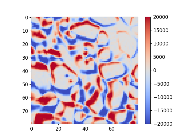
Snow image subtracted from the same image transformed by a rotation and a displacement. Blue means a negative number, grey = 0 and red is positive. See Image correlation basics for an interactive example.

We can see that there are differences between these images. However there is some alignment – the middles of some particles have low error – but there are problems on the edges. Since the amount of dark and light voxels are approximately the same in the two images that have been subtracted, the sum of this image could be expected to be close to zero.

Under this transformation, this difference is clearly not zero. If im1 and im2 have been acquired with a real measurement device which has some noise, even with the a-priori knowledge of Φ this difference will never be zero. In what follows, the objective will be to find the transformation Φ that minimises this difference as far as possible.

If we’d like to define the difference between im1 and im2, if we square the value of all the voxels in the difference, then low values will stay low, and highly negative and highly positive differences will both become highly positive. The choice of the square particular makes sense for Gaussian noise.

\[\left(\text{im1}(x) - \text{im2}(x)\right)^2\]

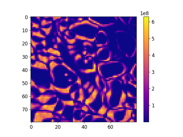
Square of Snow image subtracted from the same image transformed by a rotation and a displacement.

Here low values are well matched, and high values are poorly matched.

Image correlation – Finding Φ

Error function

We want to find Φ. Since it has 12 unknowns (4×4 = 16 components, of which the bottom row is known), this is quite a complicated problem. The first thing to do is to define an error function of Φ, which in this case is simply the classic sum of squared difference as introduced above, i.e.,

\[\mathcal{T}(\Phi) = \frac{1}{2}\sum_{x \in ROI}{\left(\text{im1}(x) - \text{im2}(\Phi \cdot x)\right)^2}\]

\(\mathcal{T}\) is a scalar function of the matrix Φ. The scalar returned is the sum-of-squares difference between im1 and im2 deformed by Φ. ROI is a 3D region-of-interest in which we are calculating this error, and for which we will now try to find Φ. Since we’re trying to measure a Φ in a small region, rather than for every voxel (which would be impossible), we have written a weak form of the solution.

Given this error function we can state our objective more clearly: we would like to find a Φ that minimises this error function. In previous work [TUD2017a] we had searched the space of displacements, rotations, etc. making small steps (line searches) to decrease the error, but what follows is much faster and more robust: we have implemented the incremental Lucas & Kanade [LUC1981] approach for image correlation. We use the formulation in homogeneous coordinates (i.e., with Φ) by the LMT in [TUD2017b], build on previous work such as [HIL2012].

Newton’s method

Assuming that im2 is differentiable, then \(\mathcal{T}\) is also differentiable, and therefore the minimisation problem becomes finding where the gradient of \(\mathcal{T}\) is zero – which is expected at a convex minimum:

\[\text{Find }\Phi\text{ such that } \nabla\mathcal{T}(\Phi) = 0\]

\(\nabla\mathcal{T}\) is a non-linear function of Φ and so we will use Newton optimisation (see Wikipedia: Newton’s method in optimization) to iteratively find the minimum of \(\mathcal{T}(\Phi)\) by small increments of Φ called \(\delta\Phi\).

Newton’s optimisation says that at iteration n the current approximation of the solution is \(\Phi^n\) and the increment to the solution \(\delta\Phi^{n+1}\) is computed as follows:

\[\nabla\mathcal{T}(\Phi^n) + \nabla^2\mathcal{T}(\Phi^n):\delta\Phi^{n+1} = 0\]

and is applied to the current solution as follows:

\[\Phi^{n+1} = \Phi^n + \delta\Phi^{n+1}\]

The objective, therefore, to be able to code this iterative procedure is to compute \(\nabla\mathcal{T}(\Phi)\) and \(\nabla^2\mathcal{T}(\Phi)\), the first and second gradients (known as Jacobian and Hessian) of the error function \(\mathcal{T}\) with respect to δΦ. In order to determine these gradients, the error function is linearised with a Talyor expansion, which simplifies the computation of the gradients. Thereafter \(\delta\Phi^{n+1}\) can be computed and iterations can now proceed.

Implementation

Regarding the implementation of this iterative procedure, we follow [TUD2017b], where this problem is recast as a matrix-vector problem, where \(\delta\Phi^{n+1}\) becomes a 12x1 vector of unknowns, the “Hessian” term to the left of it a 12x12 matrix \(M\) and on the right a 12x1 vector coming from the Jacobian \(A\), giving:

\[M^n \delta\Phi^{n+1} = A^n\]

Allowing us to solve for \(\delta\Phi^{n+1}\) as follows if the Hessian matrix is invertible:

\[\delta\Phi^{n+1} = (M^n)^{-1}A^n\]

To get a feeling for the quantities above, we can say that \(M^n\) contains the current gradient of the deformed im2 and \(A^n\) contains the difference between the im1 and the deformed im2.

Conclusion

We have a way to start with a guessed Φ and to calculate an improved approximation for Φ iteratively. It is important to note that the use of Newton’s method for minimisation means that the initial guess for Φ must be reasonably close to the right solution for this to converge.

Speaking of convergence, when should the iterative process be stopped? Classically there are two criteria:

• Either after a given number of iterations

• Or if some convergence criterion, in our case the norm of \(\delta\Phi^{(n+1)}\), becomes smaller than a given threshold

In spam, this solution is coded inside a function called register (see here). It is simple to run register directly on the example above, see: Image correlation basics. As you can see the imposed deformation of the image is recovered successfully after some iterations. The following tutorial Tutorial: Image correlation – Practice also gives an example of using the register function.

References

[HIL2012]

Hild, F., & Roux, S. (2012). Comparison of local and global approaches to digital image correlation. Experimental Mechanics, 52(9), 1503-1519. https://doi.org/10.1007/s11340-012-9603-7

[LUC1981]

Lucas, B. D., & Kanade, T. (1981). An iterative image registration technique with an application to stereo vision. https://ri.cmu.edu/pub_files/pub3/lucas_bruce_d_1981_2/lucas_bruce_d_1981_2.pdf

[TUD2017a]

Tudisco, E., Andò, E., Cailletaud, R., & Hall, S. A. (2017). TomoWarp2: a local digital volume correlation code. SoftwareX, 6, 267-270. https://doi.org/10.1016/j.softx.2017.10.002

[TUD2017b] (1,2)

Tudisco, E., Jailin, C., Mendoza, A., Tengattini, A., Andò, E., Hall, S. A., … & Roux, S. (2017). An extension of digital volume correlation for multimodality image registration. Measurement Science and Technology, 28(9), 095401. https://doi.org/10.1088/1361-6501/aa7b48