Tutorial: Refreshments in continuum mechanics

Objectives of this tutorial

This tutorial page serves as a background on the fundamental continuum mechanics concepts that are being used in different functions of spam. Thus, we will simply layout the basic equations of motion describing the change in position, orientation and shape of a material body with time. The naming of variables is consistent with [GURTIN1981].

From motion to deformation

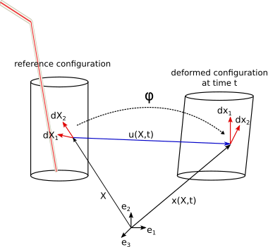
Fig. 1: Schematic of the motion between a reference and a deformed configuration

In the schematic drawing of a deformable solid cylinder, we can identify a material point by the vector describing its position in space; in the reference configuration by \(X\), and in the deformed configuration as \(x(X, t)\), assuming that a mathematical expression describing the transformation with respect to the initial position exists. Following this concept, the motion is defined by a general function which tracks the possibly complex change in spacial coordinate of the material point between the two configurations so that:

\[x=\phi(X,t)\]

If we do not have access to information on the motion of the body between two configurations, the function can be approximated by a linear displacement vector \(u(X, t)\), such that:

\[x=X+u(X,t)\]

Now, this simple relationship can very well describe the motion at every point of the body; given two configurations and a method to track a representative volume around the material points. This later requirement is detailed in the section explaining the process of correlation (see Tutorial: Image correlation – Theory.

It is here necessary to introduce the notion of deformation, as it will be used in the correlation process, by deforming local zones of interest (ZOI) to characterise the relative motion of a point with respect to its neighbours.

This requires to consider the change in orientation and length of a local vector, which is defined by the relative spacial position of two neighbouring points. In Figure 1, the vector is represented by \(dX_{1}\) in the reference configuration. In the deformed configuration, the associated vector, meaning the vector between the two exact same material points, is:

\[dx = x(X+dX,t)-x(X,t) = \frac{\partial x}{\partial X} dX + \mathcal{O}\]

ignoring higher order terms, we can write:

\[dx=FdX\]

where the tensor F is the transformation gradient tensor.

We can see that F provides richer information at the local scale than the displacement vector u alone, since it takes into account the motion of a point with respect to its neighbours. In fact, it can just as well be expressed as the differential displacement between those neighbouring points:

\[F=\frac{\partial x}{\partial X}\]

\[F=\frac{\partial (X+u)}{\partial X} = \frac{\partial X}{\partial X} + \frac{\partial u}{\partial X} = I + \frac{\partial u}{\partial X}\]

The deformation gradient F does not independently describe deformation, but rather describes a combination of both rotations and deformation. By considering the relative motion of two vectors, which are equally affected by rotation, it is possible to describe the deformation alone. Take for example the dot product of the two vectors \(dx_{1}\) and \(dx_{2}\):

\[dx_{1} \cdot dx_{2} = (F dX_{1}) \cdot (F dX_{2}) = (F^T F) dX_{1} \cdot dX_{2}\]

The tensor \(F^T F\) has the nice property of being exempt of rotation since it is symmetric. This forms the basis for the decomposition of this F tensor, as explained in details in the following section.

Transformation Gradient Tensor Decomposition

A polar decomposition theorem is used to describe the deformation as:

1. a stretching

2. followed by a rotation.

\[F = RU\]

where

• U is the symmetric right stretch tensor (acting on the reference configuration) measuring the change in the local shape, with \(U = U^T\)

• R is the orthogonal rotation tensor measuring the change of local orientation, with \(RR^T = I\), \(detR = 1\)

A rigid body motion is characterised by:

\[F = R ~~ \text{ and } ~~ U = I\]

Whereas the strain tensor characterising length and angle changes is

\[U - I\]

For a detailed explanation of the strain calculation, please head over to the tutorial Tutorial: Strain calculation

Now that we’ve introduced the fundamental role of the transformation gradient tensor F, please proceed to the next tutorial to see how it is being used into the correlation process.

[GURTIN1981]

Morton E. Gurtin (1981). An Introduction to Continuum Mechanics. Volume 158 de Mathematics in science and engineering, ISSN 0076-5392, Academic Press, 1981