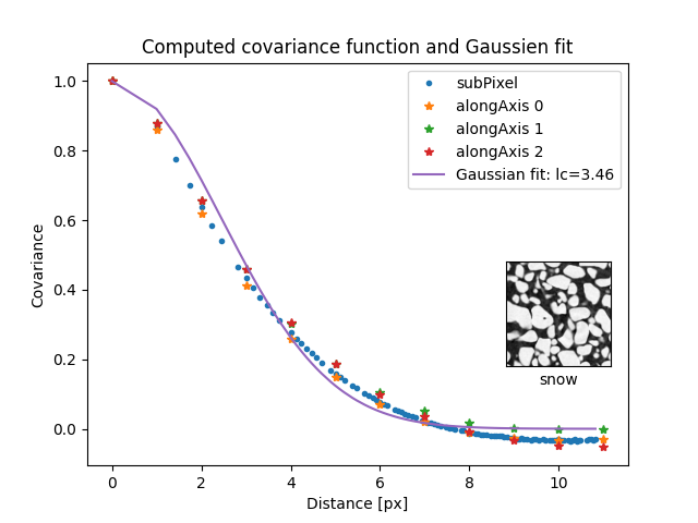
Compute covariance

This example shows how to compute the covariance of an image with two functions and how to fit it with a theoretical model.

import matplotlib.pyplot as plt
import numpy
import spam.datasets
import spam.measurements

Read the data from datasets

im = spam.datasets.loadSnow()

Compute correlation function with subPixel

A distance of 10 and a step of 2 is set to optimise the computational time

d, c = spam.measurements.covarianceSubPixel(im, distance=10, step=2, normType="first")

Compute correlation function with alongAxis

Set the integer distances, compute along the 3 axis and normalise the value with respect to the first value (variance)

h = numpy.arange(0, 12, 1)
tmp = spam.measurements.covarianceAlongAxis(im, h, axis=[0, 1, 2])
c0 = tmp[0] / tmp[0][0]
c1 = tmp[1] / tmp[1][0]
c2 = tmp[2] / tmp[2][0]

Fit the data with a Gaussian model

opt = spam.measurements.fitCovariance(d, c, functionType="gaussian")
# get the correlation length and the theoretical values
lc = opt[0]
g = spam.measurements.gaussianCovariance(d, lc)
print("Gaussian fit: lc={}".format(lc))

Gaussian fit: lc=3.46037104973026

Plot

fig, ax1 = plt.subplots()
ax1.set_title("Computed covariance function and Gaussien fit")
ax1.plot(d, c, ".", label="subPixel")
ax1.plot(h, c0, "*", label="alongAxis 0")
ax1.plot(h, c1, "*", label="alongAxis 1")
ax1.plot(h, c2, "*", label="alongAxis 2")
ax1.plot(d, g, label="Gaussian fit: lc={:0.2f}".format(lc))
ax1.set_xlabel("Distance [px]")
ax1.set_ylabel("Covariance")
ax1.legend()

# get thumbnail of the image
thumb = im[int(im.shape[0] / 2), :, :]
thumb = (thumb.astype(float) - thumb.min()) / (thumb.max() - thumb.min())
ax2 = fig.add_axes([0.70, 0.3, 0.2, 0.2])
ax2.set_xticks([])
ax2.set_yticks([])
ax2.set_xlabel("snow")
ax2.imshow(thumb, cmap="Greys_r")
plt.show()