Histogram Normalisation

This example shows how to normalise any greyscale histogram.

Histogram normalisation?

The first thing is to understand what is the process of histogram normalisation and why is it important. When dealing with tomography data, the greyscale usually ranges between 0 and 65535, but the values of the different phases differ between materials, scanning conditions, noise, structural changes on the material along the test, etc. In order to compare different scans, it is usefull to set the values of the different phases to known values that remain constant along the test. Histogram normalisation simply refers to the shift/transformation of the original histogram into one where the peak values of the phases are predefined. Several functions in spam requiere the input of normalised greyscale images, such as spam.label.localDetection() or spam.label.fixUndersegmentation(). Additionally, setting the peaks of the histogram to a predefined values enables an easy selection of the binarisation threshold: if the void peak is set at 0.25 and the solid peak is set at 0.75, the selection of 0.5 as the binarisation threshold can be considered as an objective choise.

Load data and normalise the histogram

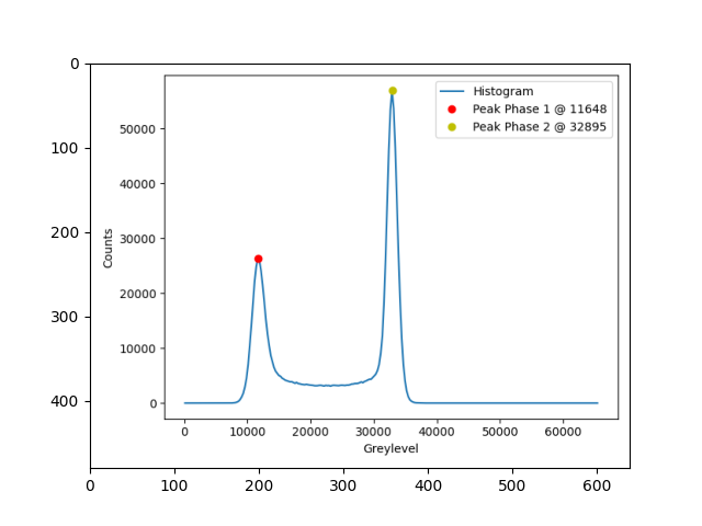
For this example we will be working with the snow dataset. Let’s load it and find the peaks of the histogram. The findHistogramPeaks requieres an initial (arbitrary) greylevel value guess that should lie between peak phase 1 and peak phase 2. This can be selected easily by looking at the histogram of the image with spam.plotting.plotGreyLevelHistogram().

import spam.datasets
import spam.helpers
import spam.plotting

snow = spam.datasets.loadSnow()
peaks = spam.helpers.histogramTools.findHistogramPeaks(snow, valley1=25000, showGraph=True, saveFigPath='./histo.png')

# begin hack:
# We saved the histogram to file to be able to show it here so that it appears on the examples gallery
import matplotlib.pyplot as plt
import matplotlib.image as img
plt.imshow(img.imread('./histo.png'))
plt.show()
# end hack

Now that we know where the peaks of the histogram are, we can apply a transformation to set them to any predefined values that we want. In this case, we are setting the void peak to be at 0.25 and the solid peak to be at 0.75. Additionally, we are setting the key cropGreyvalues to limit the range of the resulting histogram: any value outside the range [0,1] will be set to 0 or 1.

snowNorm = spam.helpers.histogramTools.histogramNorm(snow, peaks, peaksNormed=[0.25, 0.75], cropGreyvalues = [0,1])

We can check the result of the process by computing the peaks again. However we would need to change the values of the initial guess (valley1) and the greyscale range. Please note that the shape of the histogram remained the same, and we just scaled everything to fit within the range [0, 1].

peaks = spam.helpers.histogramTools.findHistogramPeaks(snowNorm, valley1 = 0.5, showGraph=True, greyRange=[0, 1])