
Note
Go to the end to download the full example code.
Multimodal registration#
A simple example to register two images acquired with different modalities
import matplotlib as mpl
import matplotlib.pyplot as plt
import numpy
import spam.datasets
import spam.deformation

import spam.DIC
import spam.helpers
Load the two images#
xr = spam.datasets.loadConcreteXr().astype("<f4")
ne = spam.datasets.loadConcreteNe().astype("<f4")

#
#
# plt.figure()
# plt.imshow(xr[halfSlice, :, :])
# plt.figure()
# plt.imshow(ne[halfSlice, :, :])
Preparation of the images#
- We start to crop the images to:
select a region of interest:
cropkeep some margin to feed the transformation:
margin
cropRatio = 0.1
crop = (
    slice(int(cropRatio * xr.shape[0]), int((1 - cropRatio) * xr.shape[0])),
    slice(int(cropRatio * xr.shape[1]), int((1 - cropRatio) * xr.shape[1])),
    slice(int(cropRatio * xr.shape[2]), int((1 - cropRatio) * xr.shape[2])),
)
cropPx = int(cropRatio * numpy.mean(xr.shape[0]))
marginRatio = 0.1
marginPx = int(marginRatio * numpy.mean(xr.shape[0]))
cropWithMargin = (
    slice(
        int((cropRatio + marginRatio) * xr.shape[0]),
        int((1 - (cropRatio + marginRatio)) * xr.shape[0]),
    ),
    slice(
        int((cropRatio + marginRatio) * xr.shape[1]),
        int((1 - (cropRatio + marginRatio)) * xr.shape[1]),
    ),
    slice(
        int((cropRatio + marginRatio) * xr.shape[2]),
        int((1 - (cropRatio + marginRatio)) * xr.shape[2]),
    ),
)
We rescale the two images between 0 and the number of bins int the joint histogram.
For sake of efficiency they have to be saved as 8bits integers (<u1).
bins = 128
xrMin = xr.min()
xrMax = xr.max()
neMax = ne.max()
neMin = ne.min()
xr = numpy.array(bins * (xr - xrMin) / (xrMax - xrMin)).astype("<u1")
ne = numpy.array(bins * (ne - neMin) / (neMax - neMin)).astype("<u1")
To see the spatial incoherency we can plot them both on the same image with a checkerbord pattern, where two adjacent squares represents the two images.
halfSlice = xr.shape[0] // 2
# checker = spam.helpers.checkerBoard(xr[halfSlice], ne[halfSlice], n=3)
# plt.figure()
# plt.imshow(checker, cmap="Greys")
# plt.colorbar()
We apply and initial guess transformation.
PhiGuess = spam.deformation.computePhi({"t": [0.0, 0.0, 0.0], "r": [15.0, 0.0, 0.0]})
tmp = spam.deformation.decomposePhi(PhiGuess)
neTmp = spam.DIC.applyPhi(ne.copy(), Phi=PhiGuess).astype("<u1")
print("Translations: {:.4f}, {:.4f}, {:.4f}".format(*tmp["t"]))
print("Rotations   : {:.4f}, {:.4f}, {:.4f}".format(*tmp["r"]))
Translations: 0.0000, 0.0000, 0.0000
Rotations   : 15.0000, 0.0000, 0.0000
Registration algorithm#
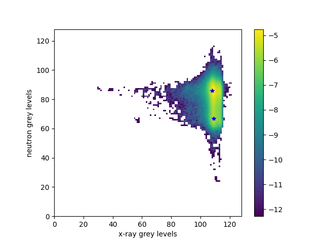
We first get the parameters of the fitted gaussians and the joint histogram. x axis corresponds to the first image grey levels. y axis corresponds to the second image grey levels. The Gaussian parameters are parameters of the two ellipsoids that fit the two peaks.
print("STEP 1: Get gaussian parameters")
nPhases = 2
gaussianParameters, jointHistogram = spam.DIC.gaussianMixtureParameters(xr[cropWithMargin], neTmp[cropWithMargin], BINS=bins, NPHASES=nPhases)
plt.figure()
tmp = jointHistogram.copy()
tmp[jointHistogram <= 0] = numpy.nan
tmp = numpy.log(tmp)
plt.imshow(tmp.T, origin="lower", extent=[0.0, bins, 0.0, bins])
plt.xlabel("x-ray grey levels")
plt.ylabel("neutron grey levels")
plt.colorbar()
for gp in gaussianParameters:
    plt.plot(gp[1], gp[2], "b*")
STEP 1: Get gaussian parameters
        im1 from 29.00 to 128.00
        im2 from 23.00 to 122.00
        p normalisation: 1.00
        Find maxima
                Min distance between maxima: 5
                00 maxima found over the 2 needed with 1.00e-01 times of the total count
                00 maxima found over the 2 needed with 1.00e-02 times of the total count
                02 maxima found over the 2 needed with 1.00e-03 times of the total count
                Maximum 1:       mu1=108.00      mu2=86.00       Phi=8.63e-03
                Maximum 2:       mu1=109.00      mu2=67.00       Phi=3.59e-03

        Phase  1:                mu1=108.00      mu2=86.00       Phi=8.63e-03
                Fit:             a=0.18  b=0.02  c=0.04  Hessian: 0.01
                Cov:             1,1=5.8691      1,2=-3.3674     2,2=30.3347

        Phase  2:                mu1=109.00      mu2=67.00       Phi=3.59e-03
                Fit:             a=0.15  b=-0.00         c=0.00  Hessian: 0.00
                Cov:             1,1=6.6323      1,2=0.8708      2,2=323.2468
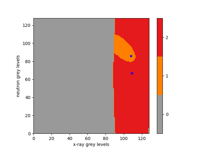
Then we create the phase diagram based on the joint histogram. Each peak corresponds to a phase (1 and 2). The grey background (points to far away from a peak) is ignored (0).
print("STEP 2: Create phase repartition")
phaseDiagram, actualVoxelCoverage = spam.DIC.phaseDiagram(gaussianParameters, jointHistogram, voxelCoverage=0.99, BINS=bins)
plt.figure()
plt.imshow(
    phaseDiagram.T,
    origin="lower",
    extent=[0.0, bins, 0.0, bins],
    vmin=-0.5,
    vmax=nPhases + 0.5,
    cmap=mpl.cm.get_cmap("Set1_r", nPhases + 1),
)
plt.xlabel("x-ray grey levels")
plt.ylabel("neutron grey levels")
plt.colorbar(ticks=numpy.arange(0, nPhases + 1))
for gp in gaussianParameters:
    plt.plot(gp[1], gp[2], "b*")
STEP 2: Create phase repartition
        9-sigma: voxel coverage = 99.15 (> 99.00%)
        8-sigma: voxel coverage = 98.99 (< 99.00%) -> Returning this phase diagram.
/home/ubuntu/spam/examples/DIC/plot_multiModalRegistration.py:125: MatplotlibDeprecationWarning: The get_cmap function was deprecated in Matplotlib 3.7 and will be removed two minor releases later. Use ``matplotlib.colormaps[name]`` or ``matplotlib.colormaps.get_cmap(obj)`` instead.
  cmap=mpl.cm.get_cmap("Set1_r", nPhases + 1),
And and we use both Gaussian parameters and phase diagram as an input of the registration algorithm
print("STEP 3: Registration")
registration = spam.DIC.multimodalRegistration(
    xr,
    ne,
    phaseDiagram,
    gaussianParameters,
    BINS=bins,
    PhiInit=PhiGuess,
    verbose=True,
    margin=marginPx,
    maxIterations=50,
    deltaPhiMin=0.005,
)
STEP 3: Registration
        Initial state        LL = 13699.66
        Iteration Number 000 LL = 13699.66 dPhi = 0.0000 Tr =  0.000,  0.000,  0.000 Ro =  15.000,  0.000,  0.000 Zo =  1.000,  1.000,  1.000
        Iteration Number 001 LL = 13531.89 dPhi = 0.0585 Tr = -0.041,  0.003,  0.041 Ro =  15.137,  0.020, -0.010 Zo =  1.000,  0.999,  0.998
        Iteration Number 002 LL = 13384.98 dPhi = 0.0550 Tr = -0.077,  0.007,  0.082 Ro =  15.282,  0.039, -0.021 Zo =  0.999,  0.997,  0.996
        Iteration Number 003 LL = 13279.62 dPhi = 0.0533 Tr = -0.115,  0.011,  0.120 Ro =  15.433,  0.059, -0.034 Zo =  0.998,  0.995,  0.994
        Iteration Number 004 LL = 13139.97 dPhi = 0.0531 Tr = -0.154,  0.015,  0.154 Ro =  15.594,  0.082, -0.044 Zo =  0.998,  0.994,  0.993
        Iteration Number 005 LL = 13046.46 dPhi = 0.0538 Tr = -0.196,  0.019,  0.187 Ro =  15.764,  0.106, -0.058 Zo =  0.997,  0.993,  0.991
        Iteration Number 006 LL = 12939.69 dPhi = 0.0549 Tr = -0.242,  0.022,  0.217 Ro =  15.938,  0.129, -0.068 Zo =  0.996,  0.992,  0.990
        Iteration Number 007 LL = 12861.05 dPhi = 0.0573 Tr = -0.292,  0.026,  0.244 Ro =  16.118,  0.151, -0.078 Zo =  0.996,  0.991,  0.989
        Iteration Number 008 LL = 12733.84 dPhi = 0.0576 Tr = -0.342,  0.030,  0.271 Ro =  16.307,  0.170, -0.090 Zo =  0.995,  0.991,  0.988
        Iteration Number 009 LL = 12623.39 dPhi = 0.0587 Tr = -0.394,  0.034,  0.296 Ro =  16.499,  0.191, -0.105 Zo =  0.994,  0.990,  0.988
        Iteration Number 010 LL = 12548.71 dPhi = 0.0623 Tr = -0.450,  0.043,  0.322 Ro =  16.698,  0.211, -0.114 Zo =  0.994,  0.990,  0.987
        Iteration Number 011 LL = 12469.26 dPhi = 0.0634 Tr = -0.507,  0.053,  0.347 Ro =  16.901,  0.231, -0.125 Zo =  0.993,  0.990,  0.987
        Iteration Number 012 LL = 12403.03 dPhi = 0.0638 Tr = -0.565,  0.064,  0.369 Ro =  17.103,  0.254, -0.133 Zo =  0.993,  0.990,  0.987
        Iteration Number 013 LL = 12341.03 dPhi = 0.0642 Tr = -0.623,  0.075,  0.391 Ro =  17.307,  0.279, -0.141 Zo =  0.992,  0.990,  0.987
        Iteration Number 014 LL = 12287.28 dPhi = 0.0613 Tr = -0.679,  0.087,  0.412 Ro =  17.506,  0.302, -0.145 Zo =  0.992,  0.990,  0.987
        Iteration Number 015 LL = 12228.45 dPhi = 0.0599 Tr = -0.733,  0.100,  0.434 Ro =  17.708,  0.325, -0.147 Zo =  0.992,  0.990,  0.987
        Iteration Number 016 LL = 12196.08 dPhi = 0.0552 Tr = -0.782,  0.113,  0.454 Ro =  17.904,  0.345, -0.143 Zo =  0.992,  0.990,  0.987
        Iteration Number 017 LL = 12155.41 dPhi = 0.0530 Tr = -0.828,  0.127,  0.474 Ro =  18.094,  0.364, -0.140 Zo =  0.992,  0.990,  0.987
        Iteration Number 018 LL = 12102.12 dPhi = 0.0485 Tr = -0.871,  0.141,  0.492 Ro =  18.273,  0.383, -0.133 Zo =  0.992,  0.991,  0.987
        Iteration Number 019 LL = 12051.18 dPhi = 0.0449 Tr = -0.909,  0.156,  0.507 Ro =  18.437,  0.402, -0.125 Zo =  0.992,  0.991,  0.988
        Iteration Number 020 LL = 12021.00 dPhi = 0.0424 Tr = -0.946,  0.171,  0.521 Ro =  18.586,  0.422, -0.116 Zo =  0.992,  0.991,  0.988
        Iteration Number 021 LL = 12014.26 dPhi = 0.0391 Tr = -0.980,  0.184,  0.535 Ro =  18.720,  0.441, -0.108 Zo =  0.992,  0.992,  0.988
        Iteration Number 022 LL = 12006.01 dPhi = 0.0350 Tr = -1.009,  0.197,  0.548 Ro =  18.841,  0.461, -0.103 Zo =  0.992,  0.992,  0.988
        Iteration Number 023 LL = 11982.48 dPhi = 0.0312 Tr = -1.035,  0.208,  0.560 Ro =  18.950,  0.477, -0.096 Zo =  0.992,  0.992,  0.988
        Iteration Number 024 LL = 11965.45 dPhi = 0.0272 Tr = -1.058,  0.217,  0.572 Ro =  19.047,  0.489, -0.091 Zo =  0.992,  0.993,  0.989
        Iteration Number 025 LL = 11948.00 dPhi = 0.0243 Tr = -1.079,  0.224,  0.581 Ro =  19.134,  0.500, -0.088 Zo =  0.992,  0.993,  0.989
        Iteration Number 026 LL = 11934.43 dPhi = 0.0221 Tr = -1.097,  0.231,  0.590 Ro =  19.210,  0.510, -0.084 Zo =  0.992,  0.993,  0.989
        Iteration Number 027 LL = 11924.29 dPhi = 0.0202 Tr = -1.115,  0.238,  0.597 Ro =  19.277,  0.519, -0.081 Zo =  0.992,  0.994,  0.989
        Iteration Number 028 LL = 11917.08 dPhi = 0.0175 Tr = -1.130,  0.243,  0.603 Ro =  19.336,  0.527, -0.077 Zo =  0.992,  0.994,  0.989
        Iteration Number 029 LL = 11912.87 dPhi = 0.0146 Tr = -1.144,  0.246,  0.608 Ro =  19.386,  0.534, -0.074 Zo =  0.992,  0.995,  0.989
        Iteration Number 030 LL = 11902.09 dPhi = 0.0130 Tr = -1.155,  0.249,  0.612 Ro =  19.428,  0.540, -0.073 Zo =  0.992,  0.995,  0.989
        Iteration Number 031 LL = 11891.75 dPhi = 0.0117 Tr = -1.166,  0.251,  0.616 Ro =  19.467,  0.546, -0.072 Zo =  0.992,  0.995,  0.989
        Iteration Number 032 LL = 11882.82 dPhi = 0.0096 Tr = -1.175,  0.253,  0.618 Ro =  19.501,  0.551, -0.072 Zo =  0.992,  0.995,  0.990
        Iteration Number 033 LL = 11869.45 dPhi = 0.0081 Tr = -1.183,  0.254,  0.619 Ro =  19.528,  0.555, -0.072 Zo =  0.992,  0.996,  0.990
        Iteration Number 034 LL = 11873.17 dPhi = 0.0064 Tr = -1.189,  0.255,  0.619 Ro =  19.552,  0.558, -0.073 Zo =  0.992,  0.996,  0.990
        Iteration Number 035 LL = 11883.93 dPhi = 0.0053 Tr = -1.194,  0.256,  0.620 Ro =  19.573,  0.560, -0.074 Zo =  0.992,  0.996,  0.990
        Iteration Number 036 LL = 11891.06 dPhi = 0.0045 Tr = -1.199,  0.256,  0.620 Ro =  19.590,  0.563, -0.075 Zo =  0.992,  0.996,  0.990

         -> Converged
Final transformation#
We can now apply the final transformation
neReg = spam.DIC.applyPhi(ne, Phi=registration["Phi"])
print("Translations: {:.4f}, {:.4f}, {:.4f}".format(*registration["transformation"]["t"]))
print("Rotations   : {:.4f}, {:.4f}, {:.4f}".format(*registration["transformation"]["r"]))
Translations: -1.1988, 0.2564, 0.6200
Rotations   : 19.5900, 0.5626, -0.0752
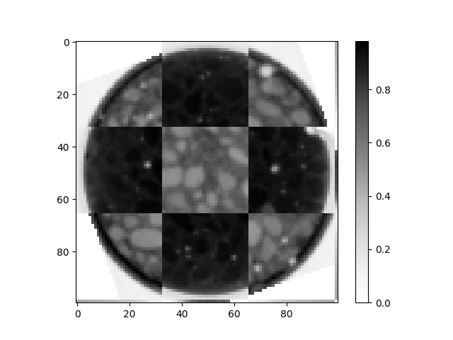
And check the validity of the result with a checkerboard pattern mixing the two images
checker = spam.helpers.checkerBoard(xr[halfSlice], neReg[halfSlice], n=3)
plt.figure()
plt.imshow(checker, cmap="Greys")
plt.colorbar()
<matplotlib.colorbar.Colorbar object at 0x7f5851c86800>
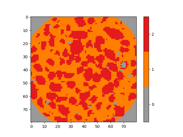
From the phase diagram a segemntation can also directly be obtained We can check that phase 1 corresponds to the mortar matrix and phase 2 to the aggregates
phaseField = registration["phaseField"]
plt.figure()
plt.imshow(
    phaseField[halfSlice, :, :],
    vmin=-0.5,
    vmax=nPhases + 0.5,
    cmap=mpl.cm.get_cmap("Set1_r", nPhases + 1),
)
plt.colorbar(ticks=numpy.arange(0, nPhases + 1))
plt.show()
/home/ubuntu/spam/examples/DIC/plot_multiModalRegistration.py:173: MatplotlibDeprecationWarning: The get_cmap function was deprecated in Matplotlib 3.7 and will be removed two minor releases later. Use ``matplotlib.colormaps[name]`` or ``matplotlib.colormaps.get_cmap(obj)`` instead.
  cmap=mpl.cm.get_cmap("Set1_r", nPhases + 1),
Total running time of the script: (0 minutes 14.602 seconds)