Scripts in spam

Spam provides scripts that tie together a number of the functions available in python. These are expected to be called from the command line (after activating your virtual environment):

$ source /path/to/spam/venv/bin/activate
(spam) $ spam-ldic -activateSomething -setSomething 5 aFileName.tif

All scripts will report all their options with a short explanation if they are simply run with - -help:

$ source /path/to/spam/venv/bin/activate
(spam) $ spam-ldic --help

Note

Almost all scripts take in images in the form of one TIFF file per state. If your 3D data is in the form of a series of slices, please save them as a single 3D TIFF file. This can be done by opening it as a stack in ImageJ/Fiji and saving directly, or loading each slice into a 3D numpy array and saving it with tifffile.imsave

Image correlation script flowchart

Below is the general flowchart for how we recommend to use the different image correlation scripts in spam. The flowchart is interactive, which means that if you click at a script name, you will be directed to its documentation.

Eye-registration script (spam-ereg)

This script performs an alignment by eye between two images. Since a direct involvement of the user is needed, the alignment is done using a graphical user interface (GUI).

The result of this eye-alignment is a single Φ (linear and homogeneous deformation function, see Tutorial: Image correlation – Theory) that maps im1 into im2.

Tip

When to use this script?

This pre-registration step can be very useful when the images are completely misaligned. Such a state could look like this:

Input:

Required

• Two TIFF greyscale images, representing the initial (im1) and the deformed (im2) configuration

Optional

• A “.tsv” file containing an initial guess of the transformation between im1 and im2

  Hint

  Make sure that the format of this file is compatible with a spam-style correlation file. (Run, for example, this script and check the result)

• --binning: Binning level (downscaling) to work with the images. Default is 1.

Output:

• A “.tsv” file containing:

  • The point where Φ is applied. This is the centre of im1

  • The components of Φ (Fzz, Fzy, Fzx, Zdisp, etc) at the used binning level. See Tutorial: Image correlation – Theory for explanation of these components

  • For compatibility reasons, information related to the iterative algorithm in spam.DIC.register() (iterations, error, deltaPhiNorm, returnStatus)

  Hint

  This file can be used as an input to other correlation scripts, like:

  • Registration script (spam-reg)

  • Pixel search script (spam-pixelSearch)

  • Regular grid local DIC script (spam-ldic)

Attention

Should we have an option to save the deformed? A “.tif” file corresponding to image 1 deformed by Φ

The script can be run like this:

1. Input files are selected through the pop-up window:

$ source /path/to/spam/venv/bin/activate
(spam) $ spam-ereg \                                            # the script

2. Input files are selected through the pop-up window and binning level is set:

$ source /path/to/spam/venv/bin/activate
(spam) $ spam-ereg \                                            # the script
         --binning 4                                            # the binning level

3. Input images are given in the terminal:

$ source /path/to/spam/venv/bin/activate
(spam) $ spam-ereg \                                            # the script
        /path/to/my/data/im1.tif /path/to/my/data/im2.tif       # the two 3D images (tiff files) to allign

4. Input images and the initial guess are given in the terminal:

$ source /path/to/spam/venv/bin/activate
(spam) $ spam-ereg \                                            # the script
        /path/to/my/data/im1.tif /path/to/my/data/im2.tif\      # the two 3D images (tiff files) to allign
        /path/to/my/data/initialPhi.tsv                         # and the initial guess

Tip

How to evaluate the result of this script?:

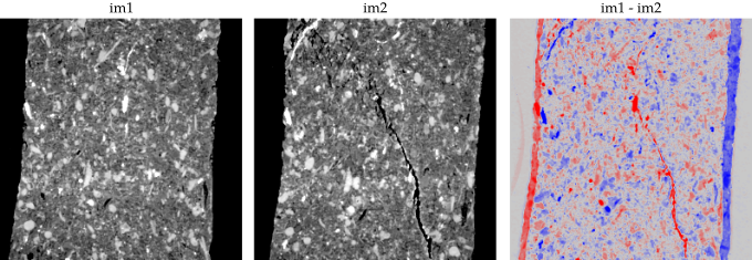
Check the greylevel residual fields. If not saved, create the deformed image 1 by running Deform image script (spam-deformImage). Compare the initial difference (im1.tif - im2.tif) and the new difference (im1Def.tif - im2.tif), which should look like this:

Are you satisfied with this alignment?

If yes, and you wish to measure the deformation between your two images, keep this Φ and move towards Registration script (spam-reg), Pixel search script (spam-pixelSearch) or Regular grid local DIC script (spam-ldic).

Registration script (spam-reg)

This script performs a non-rigid registration between two images of the same modality.

It measures a single Φ (linear and homogeneous deformation function, see Tutorial: Image correlation – Theory) that maps im1 into im2.

Tip

When to use this script?

The registration step can be very useful when there is a smooth and homogeneous deformation between the two configurations. Such a deformation could look like this:

Important

This script is actually a wraper for spam.DIC.registerMultiscale() (see here). It automatically performs a multiscale registration, starting from 4 times downscaled images propagating the result to the top scale. To change this behaviour set -bb and -be in the input parameters

Input:

Required

• Two 2D or 3D TIFF greyscale images, representing the initial (im1) and the deformed (im2) configuration

Optional

• -pf: “.tsv” file containing an initial guess of the transformation between im1 and im2.

  Hint

  This can come from Eye-registration script (spam-ereg) or a previous Registration script (spam-reg). If this guess corresponds to downscaled images, use -pfb to set the binning ratio

• -bb and -be: Binning levels (downscaling) to start (-bb) and end (-be) the multiscale procedure

  Hint

  If you do not want to downscale your images set -bb to 1. By default -be is the original scale of the input images

• -mf1: Mask of im1 defining the zones to correlate in im1. Should be a binary image (same size as im1), where False pixels are not correlated

• -m: Margin (in pixels) to allow space for interpolation and movement. Can be set different in each direction (Z, Y, X) with -m3

• -rig: Performs a rigid registration. Only translations and rotations will be measured

• -ug: Updates gradient during newton iterations inside spam.DIC.register(). More computation time but sometimes more robust and possibly fewer iterations

• -it: Regulates convergence options for spam.DIC.register(): The number of maximum iterations

• -dp: Regulates convergence options for spam.DIC.register(): The smallest change in the norm of Φ (\(\delta\Phi_{min}\))

• -o: Defines the order of greylevel interpolation; trilinear (-o 1) or cubic (-o 3)

• -g: Will plot graphs showing the progress of the registration

• -od: Defines the output directory

• -pre: Defines the prefix for the output files

• -def: Ask to save the deformed im1 at the end of the iterative algorithm. This is the measured Φ applied to im1

Output:

• A “.tsv” file containing:

  • The point where Φ was measured. This is the centre of im1 or the centre of mass of the mask (if given)

  • The components of the measured deformation function Φ (Fzz, Fzy, Fzx, Zdisp, etc). See Tutorial: Image correlation – Theory for explanation of these components

  • Information related to the iterative algorithm status (iterations, error, returnStatus, deltaPhiNorm)

  Hint

  This file can be used as an input to other correlation scripts, like:

  • Registration script (spam-reg)

  • Pixel search script (spam-pixelSearch)

  • Regular grid local DIC script (spam-ldic)

• If asked with -def: A “.tif” file corresponding to im1 deformed by the measured Φ

The script can be run like this:

$ source /path/to/spam/venv/bin/activate
(spam) $ spam-reg \                                              # the script
            /path/to/my/data/im1.tif /path/to/my/data/im2.tif\   # the two 3D images (tiff files) to correlate
            -pf /path/to/my/data/initialPhi.tsv\                 # initial guess
            -bb 2 -m 10 -def                                     # ask to start from half-sized images, set margin, ask for deformed image

Tip

How to evaluate the result of this script?:

• The registration is successful when the iterative algorithm has converged. Check returnStatus inside the “.tsv” file:

  • If returnStatus = 2: Registration converged reaching desired precision in \(\delta\Phi_{min}\)

  • If returnStatus = 1: Registration did not converge. Maximum number of iterations is reached. Retry with a higher -it or higher -dp?

  • If returnStatus = -1: Registration diverged. Error is more than 80% of previous iteration error. Retry with different binning level -bb or higher margin -m?

  • If returnStatus = -2: Registration failed. Singular matrix M (most probably image texture problem). Retry with a mask -mf1?

  • If returnStatus = -3: Registration diverged on displacement or volumetric change condition. Retry with a higher margin -m?

  • If returnStatus = -4: Registration failed. Singular \(\Phi_{min}\) matrix (most probably due to divergence). Retry with different binning level -bb? Or perhaps updating the gradient -ug?

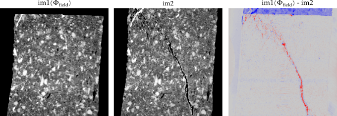
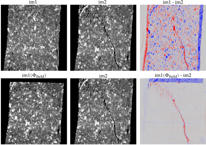
• Check the greylevel residual fields. If not asked with -def, create the deformed image 1 by running Deform image script (spam-deformImage). Compare the initial difference (im1.tif - im2.tif) and the new difference (im1Def.tif - im2.tif), which should look like this:

  

  Has the difference been decreased?

Are you satisfied with this overall deformation?

If yes, and you wish to go and look locally, keep this Φ and move towards Pixel search script (spam-pixelSearch), Regular grid local DIC script (spam-ldic) or Discrete local DIC script (spam-ddic).

Pixel search script (spam-pixelSearch)

This script performs a point-by-point “pixel search” which computes a cross-correlation of a subvolume extracted in im1 based on a brute-force search in a given search range in im2.

It measures a displacement field with a 1-pixel sensitivity that maps im1 into im2.

Tip

When to use this script?

This step can be very useful when the deformation between the two configurations is not homogeneous, meaning that it can not be captured only by a single Φ (coming from Registration script (spam-reg) for example). Such a deformation could look like this:

If you notice that there is also a homogeneous deformation (a rigid rotation for example), run Eye-registration script (spam-ereg), or Registration script (spam-reg) and pass Φ as an initial guess to this script

Important

This script can run in two different modes. It can measure a displacement field of:

1. Regularly-spaced points laid on a structured grid. See A note on the correlation grid for tips regarding the grid geometry. This mode is activated with -ns, -hws input options

2. Discrete points. For example centres of mass of particles, if your objective is to perform particle tracking. See Tutorial: Label Toolkit for more information. This mode is activated with -lab1 input option

Input:

Required

• Two TIFF greyscale images, representing the initial (im1) and the deformed (im2) configuration:

  1. If structured grid mode: The images can be 2D or 3D

  2. If discrete mode: The labelled image, which defines zones to correlate, must be given through the -lab1 input parameter. Only for 3D images for the moment. If -lab1 passed: -ns, -hws are disactivated

Optional

• -np: Number of parallel processes to use. If not passed, all the CPUs available in the system will be used

• -pf: “.tsv” file containing an initial guess of the transformation between im1 and im2

  Hint

  This can be either:

  1. A single deformation function (one-line file). This is typically the result of Eye-registration script (spam-ereg) or Registration script (spam-reg). If this guess corresponds to downscaled images, use -pfb to set the binning ratio

  2. A field of deformation functions (multiple-line file). For example, the result of a previous Pixel search script (spam-pixelSearch). Make sure that points’ positions at input file are the same as points’ positions at the current computation. Consider using Passing guess script (spam-passPhiField)

• -F: If a -pf is passed. Choose if the F part of Φ (see Tutorial: Image correlation – Theory) will be applied to the subvolume. If “rigid” only rotations are applied. If “all” everything is applied. If “no” nothing is applied.

• -sr: Search range [-Z Z -Y Y -X X] (in pixels). How far away from the point’s position in im1 should we look in im2?

  Hint

  If you provide an initial guess through -pf the search range window is around the initial guess position (this helps to avoid applying a big range of search).

• -od: Defines the output directory

• -pre: Defines the prefix for the output files

• -vtk: Ask for a vtk output for visualisation of the displacement field

For structured grid mode:

• -ns: Spacing between the grid points (in pixels). Can be set different in each direction (Z, Y, X) with -ns3

• -hws: “Half window size” (in pixels) of the correlation window. It results in a correlation window of 1+2xhws in each direction, centered at each point’s position. Can be set different in each direction (Z, Y, X) with -hws3

• -mf1: Mask of im1 defining the zones to correlate in im1. Should be a binary image (same size as im1), where False pixels are not correlated

• -mc: If -mf1 is passed. It defines the tolerance for a subvolume’s pixels to be masked before it is skipped

• -mf2: Mask of im2 defining the zones to correlate in im2. Should be a binary image (same size as im2), where False pixels are not correlated

• -glt: Grey threshold on mean values of correlation window below which the correlation is not performed (window is skipped)

• -ght: Grey threshold on mean values of correlation window above which the correlation is not performed (window is skipped)

• -tif: Ask for a tif output for visualisation of the structured displacement field

For discrete mode:

• -ld: Number of times to dilate labels before extracting them (see Tutorial: Label Toolkit)

• -lvt: Labels with volume smaller than this threshold are ignored

Output:

• A “.tsv” file containing:

  • The points position (Z, Y, X). For a structured grid mode positions are defined by the input grid. For a discrete mode positions are the centre of mass of each label

  • The displacement measured at each point

  • The correlation coefficient (pixelSearchCC) of each subvolume

  • The return status of each subvolume (returnStatus). If it is -5 the subvolume has been skipped (due to -glt, -ght or -mf1)

  • For compatibility reasons, the F part of Φ is written as the identity matrix (see Tutorial: Image correlation – Theory for explanation of the components of Φ). This is totally irrelevant to the result of this script

  • For compatibility reasons, information related to the iterative algorithm in spam.DIC.register() (iterations, error, deltaPhiNorm). These are totally irrelevant to the result of this script

• If asked with -tif or -vtk: Files for the visualisation of the displacement and correlation coefficient fields

For the structured grid mode, the script can be run like this:

$ source /path/to/spam/venv/bin/activate
(spam) $ spam-pixelSearch \                                      # the script
            /path/to/my/data/im1.tif /path/to/my/data/im2.tif \  # the two 3D or 2D images (tiff files) to correlate
            -mf1 /path/to/my/data/mask1.tif -mc 0.5 \            # the mask of im1 and the coverage to skip the subvolumes
            -pf /path/to/my/data/initialPhi.tsv -pfb 2 \         # initial guess, which was run in half-sized images
            -ns X -hws X \                                       # node spacing and half window size of the grid
            -sr -Z Z -Y Y -X X \                                 # search range
            -tif -vtk                                            # ask for tif and vtk output

For the discrete mode, the script can be run like this:

$ source /path/to/spam/venv/bin/activate
(spam) $ spam-pixelSearch \                                      # the script
            /path/to/my/data/im1.tif /path/to/my/data/im2.tif\   # the two 3D images (tiff files) to correlate
            -lab1 /path/to/my/data/lab1.tif \                    # the labelled image 1
            -pf /path/to/my/data/initialPhi.tsv -pfb 2 \         # initial guess, which was run in half-sized images
            -F rigid \                                           # apply the rigid part of the initial guess to each label
            -sr -Z Z -Y Y -X X \                                 # search range
            -vtk                                                 # ask for a vtk output

Tip

How to evaluate the result of this script?

• Check the pixelSearchCC values. A cross-correlation procedure is successful when the correlation coefficient is close to 1. Are these values low? Perhaps think of a coarser field (increase -ns)? And then pass this to the finer one through spam-passField

• Check the measured displacements. If you notice that the displacement values hit the limits of your input search range, retry by increasing this range

• Check the measured displacement fields. Do the points move as you would expect? For example you are pulling your material from the bottom edge. Do the displacement vectors point downwards increasing from the top to the bottom of your field?

• Check the greylevel residual fields. Create the deformed image 1 by running Deform image script (spam-deformImage). Compare the initial difference (im1.tif - im2.tif) and the new difference (im1Def.tif - im2.tif). It should look like this:

  

Are you satisfied with the measured displacement field?

• If mostly yes, but there are some crazy points here and there that you wish to get rid of, keep this field and move towards Filtering script (spam-filterPhiField)

• If yes, and you wish to refine it by measuring subpixel displacements, keep this Φ field and move towards Regular grid local DIC script (spam-ldic) for a structured grid mode or Discrete local DIC script (spam-ddic) for a discrete mode.

Pixel search propagate script (spam-pixelSearchPropagate)

This script performs a sequential point-by-point “pixel search” which computes a cross-correlation of a subvolume extracted in im1 based on a gaussian weighted good neighbours guess in a given search range in im2.

It measures a displacement field with a 1-pixel sensitivity that maps im1 into im2.

This script is based on https://gricad-gitlab.univ-grenoble-alpes.fr/DVC/pt4d.

Tip

When to use this script?

This can be seen as a special case of Pixel search script (spam-pixelSearch). It can be very useful when:

• There are large and not homogeneous deformations between the two configurations and

• The texture of the material is weak

Such a challenging case could look like this:

Important

This script can run in two different modes. It can measure a displacement field of:

1. Regularly-spaced points laid on a structured grid. See A note on the correlation grid for tips regarding the grid geometry. This mode is activated with -ns, -hws input options

2. Discrete points. For example:

   • “Guiding points” selected based on their strong texture. This mode is activated with -gp input option

   • Centres of mass of particles, if your objective is to perform particle tracking. See Tutorial: Label Toolkit for more information. This mode is activated with -lab1 input option

No matter the selected mode, points are ranked based on their distance to the starting point (see note below) and they are processed sequentially. This means that this script can not run in parallel.

Attention

This script requires a starting point (-sp input option), which is the first point to be tracked, and from which the propagation of the motion will start. This point should be easily tracked by eye between the two configurations. It is recommended to be either:

• A point that does not move (for example a point close to the top border for the set of images above), or

• A point that moves, but its displacement is easily measured by hand and given as an input

If the cross-correlation of this point:

• Fails (ie, correlation coefficient below given threshold -cct), the script stops. Try to give a better estimation of its displacement? Or perhaps try with another point?

• Succeeds, then continuing with its closest neighbours (see -nr and -gwd) the motion is progressively propagated by tracking the points asked (see note above)

Input:

Required

• Two TIFF greyscale images, representing the initial (im1) and the deformed (im2) configuration:

  1. If regularly-spaced mode: The images can be 2D or 3D

  2. If discrete mode: The labelled image, which defines zones to correlate, must be given, through the -lab1 input parameter. Only for 3D images for the moment. If -lab1 passed: -ns, -hws, -gp are disactivated

• -sp: Starting point [Z Y X Zdisp Ydisp Xdisp] (in pixels). The position and the displacement of the starting point

Optional

• -sr: Search range [-Z Z -Y Y -X X] (in pixels). How far away from the point’s position in im1 should we look in im2?

• -nr: Radius (in pixels) inside which to extract neighbours

• -gwd: Distance (in pixels) over which the neighbour’s distance is weighted

• -cct: Pixel search correlation coefficient threshold below which the point is considered badly correlated. This means it is not taken as a neighbour. Recommended value above 0.95

• -od: Defines the output directory

• -pre: Defines the prefix for the output files

• -vtk: Ask for a vtk output for visualisation of the displacement field

For structured grid mode:

• -ns: Spacing between the grid points (in pixels). Can be set different in each direction (Z, Y, X) with -ns3. These grid points will be ranked and then tracked based on their distance to the starting point

• -hws: “Half window size” (in pixels) of the correlation window. It results in a correlation window of 1+2xhws in each direction, centered at each point’s position. Can be set different in each direction (Z, Y, X) with -hws3

• -mf1: Mask of im1 defining the zones to correlate in im1. Should be a binary image (same size as im1), where False pixels are not correlated.

• -mc: If -mf1 is passed. It defines the tolerance for a subvolume’s pixels to be masked before it is skipped

• -mf2: Mask of im2 defining the zones to correlate in im2. Should be a binary image (same size as im2), where False pixels are not correlated

• -glt: Grey threshold on mean values of correlation window below which the correlation is not performed (window is skipped)

• -ght: Grey threshold on mean values of correlation window above which the correlation is not performed (window is skipped)

• -tif: Ask for a tif output for visualisation of the structured displacement field

For discrete mode:

• -gp: Guiding points file. A file containing points the displacement of which will be measured

  Hint

  Recommended to correspond to points with large greylevel gradients, meaning that they can be easily tracked. Typically coming from a 3D Harris Corner detection algorithm. These points are ranked based on their distance to the starting point. If passed: -ns, -hws, -lab1 are disactivated

• -ld: Only if -lab1 is passed. Number of times to dilate labels before extracting them. See Tutorial: Label Toolkit for more details

Output:

• A “.tsv” file containing:

  • The points position (Z, Y, X). For a structured grid mode positions are defined by the input grid. For a discrete mode, positions are the centre of mass of each label (if -lab1) or the guiding points (if -gp)

  • The displacement measured at each point

  • The correlation coefficient (pixelSearchCC) of each subvolume

  • The return status of each subvolume (returnStatus). If it is equal to -5 the subvolume had been skipped (due to -glt, -ght or -mf1)

  • For compatibility reasons, the F part of Φ is written as the identity matrix (see Tutorial: Image correlation – Theory for explanation of the components of Φ). This is totally irrelevant to the result of this script

  • For compatibility reasons, information related to the iterative algorithm in spam.DIC.register() (iterations, error, deltaPhiNorm). These are totally irrelevant to the result of this script

• If asked with -tif or -vtk: Files for the visualisation of the displacement and correlation coefficient fields

For the structured grid mode, the script can be run like this:

$ source /path/to/spam/venv/bin/activate
(spam) $ spam-pixelSearchPropagate \                             # the script
            /path/to/my/data/im1.tif /path/to/my/data/im2.tif \  # the two 3D or 2D images (tiff files) to correlate
            -sp Z Y X w v u \                                    # the position and displacement of the starting point
            -mf1 /path/to/my/data/im1.tif -mc 0.5 \              # the mask of im1, and the coverage to skip the subvolumes
            -nr X -gdw X \                                       # neighbour radius and gaussian distance
            -ns X -hws X \                                       # node spacing and window size of the grid
            -sr -Z Z -Y Y -X X \                                 # search range
            -cct X \                                             # correlation coefficient threshold
            -tif -vtk                                            # ask for tif and vtk output

For a discrete mode with a labelled image, the script can be run like this:

$ source /path/to/spam/venv/bin/activate
(spam) $ spam-pixelSearchPropagate \                             # the script
            /path/to/my/data/im1.tif /path/to/my/data/im2.tif \  # the two 3D images (tiff files) to correlate
            -lab1 /path/to/my/data/lab1.tif \                    # the labelled image 1
            -sp Z Y X w v u \                                    # the position and displacement of the starting point
            -nr X -gdw X \                                       # neighbour radius and gaussian distance
            -sr -Z Z -Y Y -X X \                                 # search range
            -cct X \                                             # correlation coefficient threshold
            -vtk                                                 # ask for a vtk output

For a discrete mode with a guiding points file, the script can be run like this:

$ source /path/to/spam/venv/bin/activate
(spam) $ spam-pixelSearchPropagate \                             # the script
            /path/to/my/data/im1.tif /path/to/my/data/im2.tif \  # the two 3D images (tiff files) to correlate
            -gp /path/to/my/data/guidingPoints.txt \             # the postions of the guiding points
            -sp Z Y X w v u \                                    # the position and displacement of the starting point
            -nr X -gdw X \                                       # neighbour radius and gaussian distance
            -sr -Z Z -Y Y -X X \                                 # search range
            -cct X \                                             # correlation coefficient threshold
            -vtk                                                 # ask for a vtk output

Tip

How to evaluate the result of this script?

• Check the pixelSearchCC values. A cross-correlation procedure is successful when the correlation coefficient is close to 1. Are these values low? Perhaps try with increasing -nr or -nn? Or perhaps try to track different points? For example, if in grid mode, try first with a coarser grid (increase -ns)?

• Check the measured displacements. If you notice that the displacement values hit the limits of your input search range, retry by increasing this range

• Check the measured displacement fields. Do the points move as you would expect? For example you are pulling your material from the bottom edge. Do the displacement vectors point downwards increasing from the top to the bottom of your field?

• Check the residual fields. Use the measured displacement field to deform im1. Check the initial difference (im2.tif - im1.tif) and the new difference (im2.tif - im1Def.tif).

Are you satisfied with the measured displacement field?

• If mostly yes, but there are some crazy points here and there that you wish to get rid of, keep this field and move towards Filtering script (spam-filterPhiField)

• If yes, and you wish to refine it by measuring subpixel displacements, keep this Φ field and move towards Regular grid local DIC script (spam-ldic) for a structured grid mode or Discrete local DIC script (spam-ddic) for a discrete mode.

• If yes, and you want to use this field as an inital guess to a different base, for example you measured the displacement field of a set of guiding points (with -gp) and you want to interpolate this field into a different set of points, move towards Passing guess script (spam-passPhiField).

Regular grid local DIC script (spam-ldic)

This script performs local non-rigid correlations on a structured grid. It defines a regular grid of points in im1 and runs independent correlations (calling spam.DIC.register()) for small subvolumes (or “correlation windows”) centred on each point. See A note on the correlation grid for tips regarding the grid geometry.

It measures a field of deformation functions that map each subvolume in im1 to im2.

Tip

When to use this script?

This is the final step of the procedure to get a deformation field between two configurations, where we suppose we are already close enough to the actual solution.

Such a state could look like this:

Important

This script actually runs (in parallel) spam.DIC.register() (see function) for every subvolume defined in the grid. For each local iterative algorithm to converge it is important to start close to the right solution (see Tutorial: Image correlation – Theory for more details). It is, thus, highly recommended to give an initial guess of the deformation as input to this script.

This guess can be either:

1. A single deformation function, when the deformation between im1 and im2 looks smooth and homogeneous. This is typically the result of Eye-registration script (spam-ereg) or Registration script (spam-reg)

2. A field of deformation functions, when the deformation between im1 and im2 does not look homogeneous. This field can be the result of Pixel search script (spam-pixelSearch) or a previous computation of Regular grid local DIC script (spam-ldic). Make sure that points’ positions at input file are the same as points’ positions at the current computation Consider using Passing guess script (spam-passPhiField)

Input:

Required

• Two 2D or 3D TIFF greyscale images, representing the initial (im1) and the deformed (im2) configuration

Optional

• -np: Number of parallel processes to use. If not passed, all the CPUs available in the system will be used

• -pf: “.tsv” file containing an initial guess of the transformation between im1 and im2

  Hint

  This can be either:

  1. A single deformation function (one-line file). This is typically the result of Eye-registration script (spam-ereg) or Registration script (spam-reg). If this guess corresponds to downscaled images, use -pfb to set the binning ratio

  2. A field of deformation functions (multiple-line file). The result of Pixel search script (spam-pixelSearch), or Pixel search propagate script (spam-pixelSearchPropagate) or a previous Regular grid local DIC script (spam-ldic) computation. Make sure that points’ positions at input file are the same as points’ positions at the current computation. Consider using Passing guess script (spam-passPhiField)

• -ns: Spacing between the grid points (in pixels). Can be set different in each direction (Z, Y, X) with -ns3

• -hws: “Half window size” (in pixels) of the correlation window. It results in a correlation window of 1+2xhws in each direction, centered at each point’s position. Can be set different in each direction (Z, Y, X) with -hws3

• -mf1: Mask of im1 defining the zones to correlate in im1. Should be a binary image (same size as im1), where False pixels are not correlated.

• -mc: If -mf1 is passed. It defines the tolerance for a subvolume’s pixels to be masked before it is skipped

• -glt: Grey threshold on mean values of correlation window below which the correlation is not performed (window is skipped)

• -ght: Grey threshold on mean values of correlation window above which the correlation is not performed (window is skipped)

• -m: Margin (in pixels) to allow space for interpolation for each subvolume. Since we suppose we are close to the right solution, this is typically a small value. Can be set different in each direction (Z, Y, X) with -m3

• -ug: Updates gradient during newton iterations inside spam.DIC.register(). More computation time but sometimes more robust and possibly fewer iterations

• -it: Regulates convergence options for spam.DIC.register(): The number of maximum iterations

• -dp: Regulates convergence options for spam.DIC.register(): The smallest change in the norm of Φ (\(\delta\Phi_{min}\))

• -o: Defines the order of greylevel interpolation; trilinear (-o 1) or cubic (-o 3)

• -od: Defines the output directory

• -pre: Defines the prefix for the output files

• -vtk: Ask for a vtk output for visualisation of the displacement and the iterative algorithm information fields

• -tif: Ask for a tif output for visualisation of the displacement and the iterative algorithm information fields

Output:

• A “.tsv” file containing:

  • The points position (Z, Y, X), as defined by the input grid. These are the centres of each correlation window

  • The components of the measured deformation function inside each window (Fzz, Fzy, Fzx, Zdisp, etc). See Tutorial: Image correlation – Theory for explanation of these components

  • Information related to the iterative algorithm status (iterations, error, returnStatus, deltaPhiNorm)

• If asked with -tif or -vtk: Files containing the displacement and the iterative algorithm’s information as structured fields

The script can be run like this:

$ source /path/to/spam/venv/bin/activate
(spam) $ spam-ldic \                                             # the script
            /path/to/my/data/im1.tif /path/to/my/data/im2.tif\   # the two 3D or 2D images (tiff files) to correlate
            -pf /path/to/my/data/initialPhi.tsv\                 # initial guess
            -ns X -hws X \                                       # node spacing and window size of the grid
            -glt X \                                             # set low greylevel threshold
            -dp X -it X \                                        # set convergence value for the norm of δΦ and maximum number of iterations
            -tif -vtk                                            # ask for tif and vtk output

Tip

How to evaluate the result of this script?

• Each local computation is successful when the iterative algorithm has converged. Check the returnStatus field:

  • If returnStatus = 2: Registration converged reaching desired precision in \(\delta\Phi_{min}\)

  • If returnStatus = 1: Registration did not converge. Maximum number of iterations is reached. Retry with a higher -it or higher -dp?

  • If returnStatus = -1: Registration diverged. Singular matrix M cannot be inverted. Perhaps your window size is too small?

  • If returnStatus = -2: Registration diverged. Error is more than 80% of previous iteration error. Perhaps your window size is too small?

  • If returnStatus = -3: Registration diverged on displacement or volumetric change condition. Perhaps your window size is too small? Or retry with a higher -m?

  • If returnStatus = -5: Registration skipped due to greylevel threshold condition or to mask

• Check the measured displacement fields. Do the points move as you would expect? For example you are pulling your material from the bottom edge. Do the displacement vectors point downwards increasing from the top to the bottom of your field?

• Check the greylevel residual fields. Create the deformed image 1 by running Deform image script (spam-deformImage). Compare the initial difference (im1.tif - im2.tif) and the new difference (im1Def.tif - im2.tif). It should look like this:

  

Are you satisfied with the measured deformation field?

• If mostly yes, but there are some crazy points here and there that you wish to get rid of, keep this Φ field and move towards Filtering script (spam-filterPhiField)

• If yes, and you wish directly to proceed into measuring strains, keep this Φ field and move towards Regular strain script (spam-regularStrain)

Attention

Remember to say that strains can be directly computed from decomposing the Φ of each correlation window.

Passing guess script (spam-passPhiField)

This script facilitates the manipulation of different Φ fields, applying a single deformation function to a series of points or passing a deformation field to a new basis.

Tip

When to use this script?

When you have a single deformation function (measured at one point) or field of deformation functions (measured at a set of points) and you want to apply/interpolate them to a set of new points.

Such a case could look like this:

Interpolation of a guiding points displacement field coming from Pixel search propagate script (spam-pixelSearchPropagate) (with -gp option) into the points of a structured grid

Important

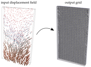
This script defines output positions based on two different modes:

1. Regularly-spaced points laid on a structured grid. See A note on the correlation grid for tips regarding the grid geometry. This mode is activated with -ns input option

2. Discrete points. For example centres of mass of particles, if your objective is to perform particle tracking. See Tutorial: Label Toolkit for more information. This mode is activated with -lab1 input option

If the input file is:

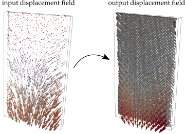
• A single deformation function: Φ is applied to each output position

• A field of deformation functions: An inverse distance interpolation of the closest (see -nr, -nn) neighbouring Φ matrices is performed

In both cases, you can choose which part of Φ (see Tutorial: Image correlation – Theory) will be passed setting the input option -m.

Input:

Required

• -pf: “.tsv” file containing the input deformation field

  Hint

  This can be either:

  1. A single deformation function (one-line file). This is typically the result of Eye-registration script (spam-ereg) or Registration script (spam-reg)

  2. A field of deformation functions (multiple-line file). For example, the result of Pixel search script (spam-pixelSearch), Pixel search propagate script (spam-pixelSearchPropagate), Regular grid local DIC script (spam-ldic), Discrete local DIC script (spam-ddic)

  If this file refers to downscaledupscaled images, use -pfb to set the correct binning ratio

Optional

• -np: Number of parallel processes to use. If not passed, all the CPUs available in the system will be used

• -F : Choose which part of Φ will be passed (see Tutorial: Image correlation – Theory) . If “all” all deformation components are passed. If “rigid” the rigid body motion is passed. If “no” only displacements are passed

• -nr: Only if input -pf is a field. Radius* (in pixels) inside which to extract neighbours for the interpolation

• -nn: Only if input -pf is a field. Number of neighbours to extract for the interpolation. Disactivates -nr

• -rst: Only if input -pf is a field. Return status threshold below which input points are not taken as neighbours

• -od: Defines the output directory

• -pre: Defines the prefix for the output files

• -vtk: Ask for a “.vtk” output for visualisation of the displacement field

For structured grid mode:

• -ns: Spacing between the grid output points (in pixels). Can be set different in each direction (Z, Y, X) with -ns3

• -im1: The image on which to define the grid. If passed, -im1shape is not needed

• -im1shape: The shape of the image [Z Y X] (in pixels) on which to define the grid. If passed, -im1 is not needed

• -tif: Ask for a “.tif” output for visualisation of the displacement field

For a discrete mode:

• -lab1 The labelled image (see Tutorial: Label Toolkit) from which the output positions are calculated (centres of mass of labels)

Output:

• A “.tsv” file containing:

  • New positions (Z, Y, X), as defined by the input grid (-ns) or the labelled image (-lab1)

  • The components of the applied or interpolated deformation function (Fzz, Fzy, Fzx, Zdisp, etc). Option -m defined which part of Φ was passed

  • For compatibility reasons, information related to the iterative algorithm in spam.DIC.register() (iterations, error, deltaPhiNorm, returnStatus). These are totally irrelevant to the result of this script

• If asked with -tif or -vtk: Files containing the displacement field

For output points defined by a labelled image, the script can be run like this:

$ source path/to/spam/venv/bin/activate
(spam) $ spam-passPhiField                       # the script
            -pf /path/to/my/data/Phi.tsv\        # the file containing the correlation result (let's assume it's a single-line registration)
            -F "all"                             # pass all components of Φ
            -lab1 /path/to/my/data/lab1.tif\     # path to labelled image to define the output points
            -vtk                                 # ask for a VTK output

…and it simply applies the result of a registration to the centres of mass of a labelled image.

For output points defined in a structured grid, the script can be run like this:

$ source path/to/spam/venv/bin/activate
(spam) $ spam-passPhiField                       # the script
            -pf /path/to/my/data/PhiField.tsv\   # the file containing the correlation result (let's assume it's a field)
            -F "no"                              # pass only disp
            -im1 /path/to/my/data/im1.tif\       # path to image to define the output grid
            -ns X \                              # node spacing of the output grid
            -nr X \                              # radius to extract neighbours for the interpolation (since we passed a field)
            -tif -vtk                            # ask for TIFF file and VTK output

Tip

The result of this script could look like this:

Displacement field of guiding points coming from Pixel search propagate script (spam-pixelSearchPropagate) (with -gp option) interpolated into a structured grid

Filtering script (spam-filterPhiField)

This script corrects or filters a deformation field.

Tip

When to use this script?

• When you are generally satisfied with your deformation field, but there are some crazy points that you would like to get rid of. Such a field could look like this:

  

  Displacement and return status fields coming from Regular grid local DIC script (spam-ldic)

• It is recommended to use this script before calculating strains.

Attention

Only one operation is allowed at a time. This means that you can either ask for correction OR filtering of your input field. You can for example:

1. Run a first computation for correcting badly correlated points and

2. If satisfied with the correction, give the resulted field as a new input to this script asking now for an overall filtering of the corrected field.

Important

If the correction of the field is asked, this script first selects bad points based on different metrics and then corrects them.

The selection of bad points can be based on one of the following metrics:

• The return status, activated with -srs

  A point’s return status is the result of Regular grid local DIC script (spam-ldic) or Discrete local DIC script (spam-ddic). A return status equal to 2 means that the local algorithm inside spam.DIC.register() has converged. A threshold below which points are considered bad can set with -srst.

• The correlation coefficient, activated with -scc

  A point’s correlation coefficient is the result of Pixel search script (spam-pixelSearch) or Pixel search propagate script (spam-pixelSearchPropagate). Typically a point with a coefficient greater than 0.99 is considered as successfully correlated. A threshold below which points are considered bad can be set with -scct.

• The local coherency, activated with -slqc

  As per per Masullo and Theunissen 2016, a point’s local coherency is the average residual between the point’s displacement and a second-order parabolic surface, fitted to the point’s closest N neighbours and evaluated at the point’s position. The estimation of the local coherency is implemented in spam.DIC.estimateLocalQuadraticCoherency() and is based on https://gricad-gitlab.univ-grenoble-alpes.fr/DVC/pt4d. Typically, a point with a coherency value smaller than 0.1 is classified as coherent. Thus, no input coherency threshold is allowed.

The correction of bad points can be done with one of the following operations:

• Inverse distance weighting of closest good neighbours, activated with -cint

• Local quadratic fit of closest good neighbours, activated with -clqf

Closest neighbours are selected based on distance -nr or number -nn.

This script filters the input field based on:

• An overall median filter, activated with -fm with a given radius -fmr. You can choose to filter all components of Φ ( -F all ) or only the displacements ( -F no).

For both correction and filtering, this script by default ignores background points based their return status (i.e, returnStatus=-5). If you want to change this behaviour see -nomask input option.

Input:

Required

• -pf: “.tsv” file containing the deformation field.

  This file can come either from Pixel search script (spam-pixelSearch), Pixel search propagate script (spam-pixelSearchPropagate), Regular grid local DIC script (spam-ldic), Passing guess script (spam-passPhiField) or Filtering script (spam-filterPhiField). If this file refers to downscaled/upscaled images, use -pfb to set the correct binning ratio

Optional

• -np: Number of parallel processes to use. If not passed, all the CPUs available in the system will be used

• -nomask: If activated, correlation points in background (i.e, with returnStatus*=-5) will **not* be ignored from the correction/filtering operations. It is recommended not to activate this option

• -nr: Radius (in pixels) inside which to extract neighbours for field interpolation. Disactivates -nn

• -nn: Number of neighbours to extract for field interpolation. Disactivates -nr

• -srs: Selects bad points based on their correlation return status. See -srst for setting the threshold. Disactivates -scc, -slqc, and -fm

• -srst: Return status threshold below which points are considered bad. Default behaviour selects points with RS<=1

• -scc: Selects bad points based on their correlation coefficient. This is for fields coming from Pixel search script (spam-pixelSearch), Pixel search propagate script (spam-pixelSearchPropagate). See -scct for setting the threshold. Disactivates -slqc

• -scct: Correlation coefficient threshold below which points are considered bad. Default behaviour selects points with CC<=0.99

• -slqc: Selects bad points based on their local quadratic coherency value. Default behaviour selects points with coherency bigger or equal to 0.1. This threshold is not modifiable

• -cint: Corrects selected bad points by an interpolation of the extracted neighbours’ Φ with weights equal to the inverse of the distance. See -F to select the interpolated components

• -F: Choose which part of Φ (see Tutorial: Image correlation – Theory) will be corrected/filtered. If “all” all deformation components are considered (default behaviour). If “rigid” the rigid body motion is considered. If “no” only displacements are considered

• -clqf: Corrects selected bad points based on local quadratic fit of the extracted neighbours. The filt only applies to the displacement vector

• -fm: Activates an overall median filter on the deformation field. -F can be set either as “all” or as “no”. The filtering operation is allowed only if none of -scc, -slqc or -slqc is passed

• -fmr: Sets the radius (in pixels) of the median filter. Default behaviour is a radius of 1 pixel

• -od: Defines the output directory

• -pre: Defines the prefix for the output files

• -vtk: Ask for a vtk output for visualisation of the displacement field

• -tif: Ask for a tif output for visualisation of the displacement field

Output:

• A “.tsv” file containing:

  • The points position (Z, Y, X) which are the same as the input field

  • The components of each point’s deformation function (Fzz, Fzy, Fzx, Zdisp, etc). See Tutorial: Image correlation – Theory for explanation of these components. Deformation components of good and background points are not modified

  • Information related to the iterative algorithm status (returnStatus, iterations, etc). Values of good and background points are not modified. returnStatus of corrected/filtered bad points is set equal to 1

• If asked with -tif or -vtk: Files containing the corrected/filtered deformation fields

For a correction operation the script can be run like this:

$ source path/to/spam/venv/bin/activate
(spam) $ spam-filterPhiField                     # the script
            -pf /path/to/my/data/PhiField.tsv\   # the file containing the deformation field
            -srs -srst 1\                        # select bad correlation points based on return status equal or less than 1
            -nn X\                               # extract closest X good neighbours
            -cint -F "no"\                       # correct displacements of bad points based on an inverse weighted distance interpolation of extracted good neighbours displacements
            -tif -vtk                            # ask for TIFF file and VTK outputs

For a filtering operation the script can be run like this:

$ source path/to/spam/venv/bin/activate
(spam) $ spam-filterPhiField                     # the script
            -pf /path/to/my/data/PhiField.tsv\   # the file containing the deformation field
            -fm -fmr X -F "all"\                 # ask for a median filter of the input displacements with a radius of X px
            -tif -vtk                            # ask for TIFF file and VTK outputs

Tip

The result of this script could look like this:

Are you satisfied with the corrected/filtered displacement field?

• If no, retry by increasing -nr or -nn or -fmr?

• If yes, and you wish to run a last correlation step, keep this Φ field and move towards Regular grid local DIC script (spam-ldic)

• If yes, and you wish to proceed into measuring the strains, keep this Φ field and move towards Regular strain script (spam-regularStrain)

Regular strain script (spam-regularStrain)

This script calculates the strain field between two configurations, based on a displacement field measured at a regular grid.

Important

This script calculates strains based on three modes:

1. Geers (see Tutorial: Strain calculation), default option

2. Q8 (see Tutorial: Strain calculation), activated with -cub

3. raw (see Tutorial: Strain calculation), activated with -raw

For further details regarding the strain calculation in spam (i.e., formulation, invariants), please see the detailed tutorial here Tutorial: Strain calculation.

Input:

Required

• a “.tsv” file containing the deformation field. This file can come either from spam-pixelSearch or spam-ldic

Optional

• -r: Only for Geers mode. The radius (in units of the grid spacing) inside which to select neighbours

• -cub: Activates Q8 mode

• -raw: Calculates the deformation gradient tensor F directly from the correlation window instead of computing it from the displacement field (as happens in Geers or Q8 mode)

• -rst: Return status threshold below which points are ignored for the strain calculation. Default behaviour selects points with RS>1

• -nomask: If activated, no correlation points ignored from the strain calculation. It is recommended not to activate this option

• -comp: Defines which strain components to return (see Tutorial: Strain calculation)

• -od: Defines the output directory

• -pre Defines the prefix for the output files

• -vtk: Ask for a vtk output for visualisation of the strain field

• -tif: Ask for a tif output for visualisation of the strain field

Output:

• A “.tsv” file containing:

  • The points position (Z, Y, X), where the strain was measured. It is the centre of the correlation window for Geers and -raw mode.

  • The strain components

• If asked with -tif or -vtk: Files containing the strain components as structured fields

The script can be run like this:

$ source path/to/spam/venv/bin/activate
(spam) $ spam-regularStrain                    # the script
            /path/to/my/data/PhiField.tsv\     # the file containing the correlation result
            -comp vol dev\                     # ask for first and second invariants of strain
            -tif -vtk                          # ask for TIFF file and VTK output of the strain field

Deform image script (spam-deformImage)

This script deforms an image based on a given deformation.

Tip

When to use this script?

When you measured a deformation between two configurations and you want to apply it to your initial configuration (or im1) and see how it is deformed:

Greylevel images and their measured displacement field coming from Pixel search script (spam-pixelSearch) after being filtered by running Filtering script (spam-filterPhiField)

Important

The input deformation file can be:

• A single deformation function: The measured Φ matrix is used to map each voxel position from the initial to the deformed configuration (x’ = Φx)

• A field of deformation functions: The displacement part of the Φ field is used to triangulate (using CGAL) the displaced measurement positions and interpolate the greyvalue of each voxel

Input:

Required

• A TIFF greyscale image, representing the initial (im1) configuration that will be deformed

• -pf: “.tsv” file containing the input deformation field

  Hint

  This can be either:

  • A single deformation function (one-line file). This is typically the result of Eye-registration script (spam-ereg) or Registration script (spam-reg)

  • A field of deformation functions (multiple-line file). For example, the result of Pixel search script (spam-pixelSearch), Pixel search propagate script (spam-pixelSearchPropagate) or Regular grid local DIC script (spam-ldic)

  If this file refers to downscaled/upscaled images, use -pfb to set the correct binning ratio

Optional

• -rr: Only if input -pf is a single matrix. Deforms the image using only the rigid part of Φ (only translations and rotations)

• -a: Only if input -pf is a field. CGAL Alpha value for triangulation cleanup (negative = auto, zero = no cleanup, positive = userval)

• -rad: Only if input -pf is a field. Exclude points outside a given radius. Assumes a cylinder with the axis in z-direction

• -od: Defines the output directory

• -pre Defines the prefix for the output file

Output:

• A “.tif” file corresponding to im1 deformed by the input deformation file

The script can be run like this:

$ source path/to/spam/venv/bin/activate
(spam) $ spam-deformImage                        # the script
            /path/to/my/data/im1.tif             # the 3D image (tiff file) to be deformed
            -pf /path/to/my/data/PhiField.tsv\   # the file containing the deformation file
            -r X                                 # the radius to exclude points from the triangulation

Tip

It is highly recommended to use this script to calculate greylevel residual fields and evaluate any of your correlation steps:

Greylevel images and their residual fields before (top) and after (bottom) a correlation

A note on the correlation grid

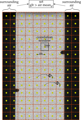
A small note on the choice of the input options -ns and -hws would be useful. Generally, the size of the correlation window (2× hws +1) and the spacing of the measurement points (ns) can be chosen independently, by selecting a spacing smaller than the window size (overlapping windows), equal to the window size (contiguous windows) or bigger than the window size (separate windows). Note that contiguous correlation windows will ensure statistical independence of the corresponding error.

As for the choice of the number of the measurement points (defined by -ns), it should be kept in mind that there is a clear trade-off between the spatial resolution of the measurement (node spacing) and the level of the measurement uncertainty. A complex heterogeneous kinematic field requires many measurement points in order to be accurately described at the expense, though, of higher uncertainties which can dominate the signal for very small windows. A compromise is therefore needed, which is strongly related to the particular experiment conducted, the material studied and the scale of the mechanisms of interest.

An illustration of a regular grid (in 2D) with contiguous correlation windows is given below. The image is the reference configuration of the V4 data set – an x-ray tomography of a sandstone performed before and after straining done by E. Charalampidou and used as an example in TomoWarp 2 [TUD2017a]. You can download VEC4.zip from spam tutorial archive on zenodo.

Example of a regular grid with spacing of the measurement points (ns) double of the half-window size (hws), so as not to have overlapping correlation windows. A linear deformation function Φ is calculated independently at the centre of each correlation window

Note that in this case a -glt 20000 is recommended to avoid correlating the windows that fall on the sides of the specimen (surrounding air). To calculate the deformation field between V4_01.tif and V4_02.tif measured on the regular grid shown in the image above, only very simple lines are needed:

Discrete local DIC script (spam-ddic)

A script for performing kinematical measurements on discretely defined objects is provided with spam-ddic. The objects to correlate are defined in a labelled volume as individually-numbered objects (see Tutorial: Label Toolkit and Tutorial: Discrete Image correlation). By default, the extent of each label is used to mask the greylevels that are correlated (see spam.label.boundingBoxes). The result of running this script is an independent measurement of a linear deformation function \(\Phi\) (see Tutorial: Image correlation – Theory) at the centre of mass of each object.

Inputs

At the very least this script must be run with three TIFF images in this order:

1. A greyscale image of state 1

2. A labelled image of state 1

3. A greyscale image of state 2

Here is an example of the vertical slices through the “Martian Simulant” M2EA05 dataset from [Kawamoto2016] that will be used for discrete correlation.

Example of input images for a discrete correlation. A linear deformation function Φ is calculated independently at the centre of mass of each labelled object

Other key input options are:

• -ld sets how many iterations of dilation will be applied to each object to extract the greylevels to correlate

• -regbb and -regbe to perform an initial multiscale registration of the two provided images – this is highly recommended. In many cases (without too complicated and large displacement fields), this step can avoid the need to perform a computationally expensive pixel search. -regbb defines the initial binning level -regbe defines the final binning level.

• -vt the volume (in voxels) of the smallest object to correlate.

• -lci and -lcp regulate convergence options for each grid point spam.DIC.registration.register run in an object: the number of maximum iterations and the smallest change in the norm of Φ (\(\delta\Phi_{min}\)) respectively.

• -od and -pre set the output directory and the prefix for the output files respectively.

As per the spam-ldic script, a large number of other options exist and can be seen with - -help.

For 3D images, only a single 3D TIFF per state file is supported for the moment. This script can run in parallel using the MPI multiprocessing library as above.

Outputs

By default the outputs of a discrete correlation are:

• a TSV file with the transformation and correlation status for each object

• a VTK file with the displacement vectors of each object

The code will return, for each label, the following information:

• The label number

• The label’s Z,Y,X position (centre of mass)

• The measured label’s Z,Y,X displacement

• The measured label’s components of F matrix

• The correlation error for this label: final difference in greylevels between im1 and im2(\(\Phi\).x) subvolumes with a normalisation applied.

• The number of iterations until convergence (equal to -lci if convergence was not reached)

• The return status (this is important!):

  • 2 = Convergence: reached desired \(\delta\Phi_{min}\) (-lcp input)

  • 1 = Not Convergence: stopped by hitting the maximum number of iterations (-lci input) without diverging

  • -1 = Divergence: error is more than 80% of previous iteration error (see spam.DIC.registration.register)

  • -2 = Iterative procedure stopped: singular matrix M cannot be inverted (see spam.DIC.registration.register)

  • -3 = Divergence: diverged on displacement or volumetric change condition (see spam.DIC.registration.register)

  • -4 = Margin alignment for im1 and im2 subvolumes failed (the iterative procedure never started)

  • -5 = Failed margin alignment (too close to edge?) or failed volume condition

  • -6 = Not used right now

  • -7 = Label missing or NaNs/infinite in Phi

As per spam-ldic script, to perform a discrete correlation between these two M2EA05 states, again only very simple lines are needed:

$ source path/to/spam/venv/bin/activate
(spam) $ spam-ddic                                            # the script
            data/M2EA05/M2EA05-quart-01.tif \                 # reference greyscale image
            data/M2EA05/M2EA05-quart-01-bin-watershed.tif \   # reference labelled image
            data/M2EA05/M2EA05-quart-02.tif \                 # deformed greyscale image

To see the output of this script please go to the detailed tutorial for discrete image correlation here Tutorial: Discrete Image correlation.