Orientations toolkit examples

Here we present some of the functions of the orientations toolkit, specifically on how to create vectorial data and analyse it in different ways

Generation of a distribution of vectors

Let’s start by creating two different set of vectors: i) an isotropic distribution (i.e., vectors pointing in every direction in space), and ii) a distribution with a prefered orientation. For creating the isotropic distribution:

import numpy
import spam.orientations
N = 2000 # Number of vectors, same for both subsets
subset1 = spam.orientations.generateIsotropic(N)

For the second subset, we need to set a mean orientation and a concentration parameter. This is performed by modeling the data using a von Mises-Fisher distribution. This statistical distribution is specially suited for directional data, and is analogous to a multivariate Gaussian distribution. The VMF distribution presents a rotation symmetry around a mean orientation, while the tightness around it is characterised by the concentration parameter kappa (higher values of kappa imply a larger concentration towards the mean orientation). Let’s create the second subset with an imposed orientation and concentration parameter

inclination = numpy.radians(45) # Angle of the vector with the Z axis
azimuth = numpy.radians(0) # Angle of the vector in the XY plane
mu = numpy.reshape([numpy.cos(inclination),
                    numpy.sin(inclination)*numpy.sin(azimuth),
                    numpy.sin(inclination)*numpy.cos(azimuth)],(1,3))
kappa = 6 # Concentration parameter
subset2 = spam.orientations.generateVonMisesFisher(mu, kappa, N)

Visualize the data

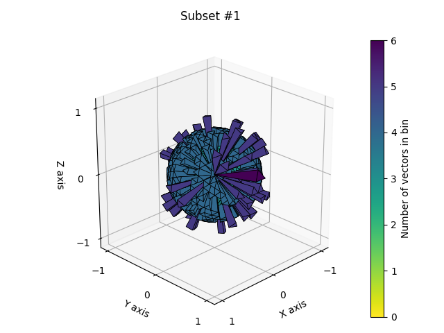
There are several ways to observe the raw vectorial data. Here we will use two different methods. Let’s first take a look at the raw vectorial data in 3D, plotting the spherical histogram of each subset

import spam.plotting
spam.plotting.orientationPlotter.plotSphericalHistogram(subset1, title='Subset #1', verbose=False)
spam.plotting.orientationPlotter.plotSphericalHistogram(subset2, title='Subset #2', verbose=False)

• 
• 

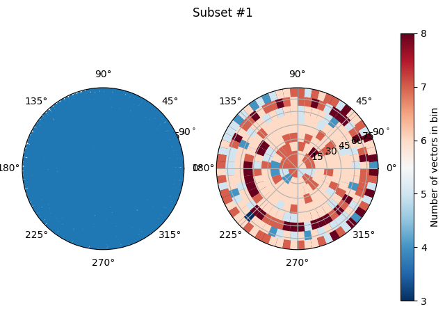
Additionally, we can use the orientation plotter, projecting the vectors into a 2D plane.

spam.plotting.orientationPlotter.plotOrientations(subset1, title='Subset #1')
spam.plotting.orientationPlotter.plotOrientations(subset2, title='Subset #2')

• 
• 

Analyze the data

Once we have the distributions, lets compute a fabric tensor and check how anisotropic are both subsets.

nSub1, fSub1, aSub1 = spam.orientations.fabricTensor(subset1)
nSub2, fSub2, aSub2 = spam.orientations.fabricTensor(subset2)
print('\n Subset #1 fabric anisotropy: {}'.format(aSub1))
print('\n Subset #2 fabric anisotropy: {}'.format(aSub2))

Subset #1 fabric anisotropy: 0.02856137401137532

Subset #2 fabric anisotropy: 4.3839916285594045

Here it is easy to see that the anisotropy of the first subset is very low (pointing to an homogenous distribution of vectors), while the high value of anisotropy for the second subset points to the existance of a preferred orientation. Lets plot the deviatoric part of the fabric tensors

spam.plotting.orientationPlotter.distributionDensity(fSub1, title='Subset #1')
spam.plotting.orientationPlotter.distributionDensity(fSub2, title='Subset #2')

• 
• 

Finally, we can try to fit a von Mises Fisher distribution to the second subset check its parameters

vMFsubset2 = spam.orientations.fitVonMisesFisher(subset2)
print('Mean orientation: {}'.format(vMFsubset2['mu']))
print('Inclination: {}'.format(vMFsubset2['theta']))
print('Azimuth: {}'.format(vMFsubset2['alpha']))
print('Kappa: {}'.format(vMFsubset2['kappa']))

Mean orientation: [0.713 0.025 0.7  ]
Inclination: 44.48213333247687
Azimuth: 2.040130920484964
Kappa: 6.053049520017291