Labelled image toolkit simple examples

Here we demonstrate some of the simple functions of the labelled toolkit, to deal with discrete materials

import matplotlib.pyplot as plt
import numpy
import spam.mesh
import spam.label
import spam.plotting
import spam.datasets
import scipy.ndimage

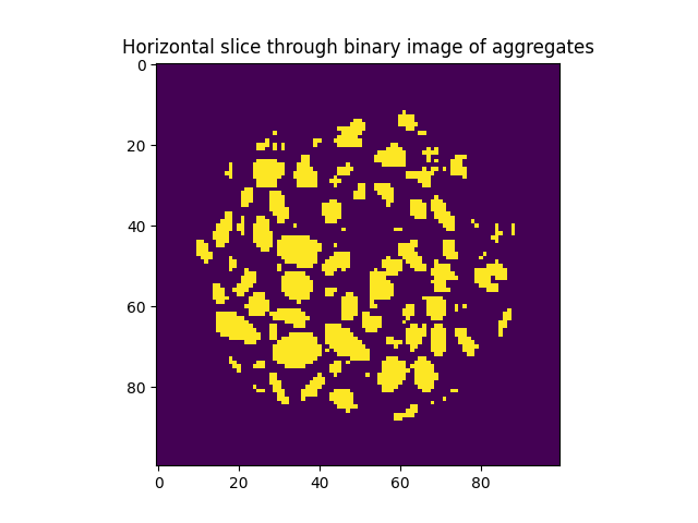
Prepare a binary image

Load concrete data with neutrons, and extract only the aggregates. This is done with an initial top-and-bottom threshold, combined with a cylindrical mask, and dilated aggregates in order to compensate partial volume effect

im = spam.datasets.loadConcreteNe()
midSlice = im.shape[0] // 2

# Top and bottom threshold to catch aggregates
binary = numpy.logical_and(im > 28000, im < 40000)

# Define a cylinder, to remove floating outside of specimen
cyl = spam.mesh.createCylindricalMask(im.shape, 40)

# Keep only the intersection of cylinder and "binary"
binary = numpy.logical_and(binary, cyl)

# Identify and dilate Pores
pores = scipy.ndimage.binary_dilation(im < 26000, iterations=1)

# Remove pores from binary image
binary[pores] = 0

plt.figure()
plt.title("Horizontal slice through binary image of aggregates")
plt.imshow(binary[midSlice])

<matplotlib.image.AxesImage object at 0x7f15b17ca390>

Separate and label individual particles

Starting with this binary image, we will use ur interface to the ITK watershed in order to obtain an image where the binary phase is split into multiple uniquely numbered segments – a labelled image

labelled = spam.label.ITKwatershed.watershed(binary)

print("{} particles have been identified".format(labelled.max()))
plt.figure()
plt.title("Horizontal slice through labelled image of aggregates")
plt.imshow(labelled[midSlice], cmap=spam.label.randomCmap)

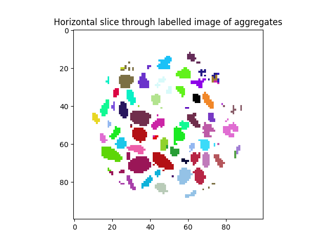
540 particles have been identified

<matplotlib.image.AxesImage object at 0x7f15b1f60e50>

It’s important to understand that each colour in this slice represents a different integer value, meaning the all voxels with the same value represent the same particle.

Typically labels are numbered from top to bottom. Label 0 is typically the background. We don’t do any computations on this zero-label, but we keep it in the outputs so that volumes[1] gives the volume of label number 1

Label toolkit: Volumes

Start with basic measurements: the most simple thing that can be done is probably counting the number of voxels that each label is made up of, which is simply counting the number of occurrences of each label value.

The result of volumes is a vector (whose length is the number of labels+1) containing the number of voxels counted for each label. The same thing could be obtained (a little slower) using numpy.unique(labelled, return_counts=True)

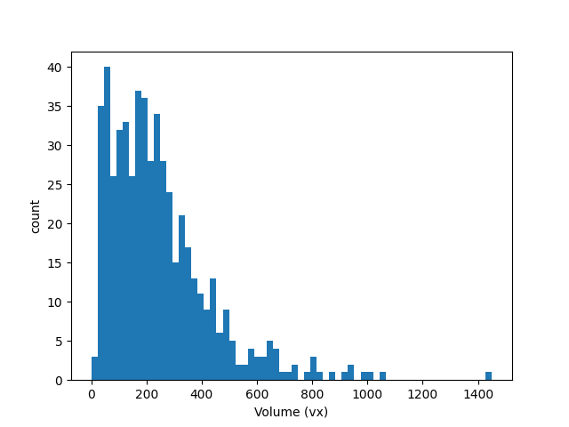
Let’s compute the volumes of each particle and draw the distribution of particle volumes:

volumes = spam.label.volumes(labelled)
print(volumes.shape)

plt.figure()
plt.hist(volumes, bins=64)
plt.xlabel("Volume (vx)")
plt.ylabel("count")

(541,)

Text(47.097222222222214, 0.5, 'count')

The output mentions the calculation of bounding boxes, before the computation of the volumes of each particle. Let’s see what these are…

Label toolkit: Bounding Boxes

Bounding boxes are simply a description of the smallest box, aligned with Z Y X directions that each label can fit inside.

They are particularly convenient to limit the memory space for computations performed on labels. Here we will now compute them and save them inside a variable, which we can recycle when we call other functions (please note that when we called volumes above without passing it the bounding boxes, they were computed on-the-fly.

The boundingBoxes variable will contain 6 numbers for each label: Zmin, Zmax, Ymin, Ymax, Xmin, Xmax.

scipy.ndimage.find_objects works the same way, but is considerably slower.

boundingBoxes = spam.label.boundingBoxes(labelled)
print(boundingBoxes)

[[ 0  0  0  0  0  0]
 [ 1  6 49 53 47 59]
 [ 2 10 57 66 13 23]
 ...
 [85 94 61 73 24 34]
 [89 95 78 85 65 74]
 [90 94 48 60 50 63]]

Label toolkit: Centres of Mass

The centre of mass of each particle can also be computed with ease. the centresOfMass function can take as input the bounding boxes that we just computed in order to avoid re-computing them.

The output of this function is a floating point number for the position of the centre of mass of each label.

This is simply a spatial average of the Z, Y and X positions of the voxels that make up each label. The fact that there is an averaging procedure means that the positioning can be quite precise and accurate.

We consider the centre of mass of a single voxel at 0,0,0 to be at 0.5, 0.5, 0.5, i.e, we consider voxels to be indexed on the top-left-back position.

centresOfMass = spam.label.centresOfMass(labelled, boundingBoxes=boundingBoxes)
print(centresOfMass)

[[ 0.     0.     0.   ]
 [ 4.038 50.885 55.058]
 [ 5.36  61.779 18.61 ]
 ...
 [91.    65.843 28.4  ]
 [91.825 80.738 70.325]
 [92.432 53.185 54.907]]

Label toolkit: Moment of Inertia

The moment of inertia (or “second moment of area”) translates the shape of the particle.

The output of this function is the [maximum, middle, minimum] eigenValues and [maximum, middle, minimum] eigenVectors of the moment of inertia tensor for each label.

The eigenVectors are of particular interest because they point in the direction of the [ shortest, intermediate, longest ] axes of the label. In the case of very symmetric shapes, this does not work very well – in the case of a cube or a cylinder these axes tend to point in the direction of the edges. There are defined with Z Y X components.

The eigenValues are related to the lengths of the axes, but not directly, we will use another function to obtain the lengths of the axes lower.

The momentOfInertia allows boundingBoxes and centresOfMass to be provided.

MOIeigenValues, MOIeigenVectors = spam.label.momentOfInertia(labelled, boundingBoxes=boundingBoxes, centresOfMass=centresOfMass)
print(MOIeigenVectors)

[[ 0.     0.     0.    ...  0.     0.     0.   ]
 [-0.705 -0.676  0.213 ... -0.348  0.068 -0.935]
 [-0.176  0.764 -0.621 ...  0.258 -0.573 -0.778]
 ...
 [ 0.285  0.46  -0.841 ...  0.947 -0.272  0.172]
 [-0.746 -0.65  -0.149 ... -0.169  0.4   -0.901]
 [ 0.964 -0.167 -0.206 ...  0.085 -0.542  0.836]]

Now we can use the orientation plotter to show the 3D orientation of the long axes of each label (starting from label 1).

spam.plotting.orientationPlotter.plotOrientations(MOIeigenVectors[1:, 6:9], plot='bins', numberOfRings=5)

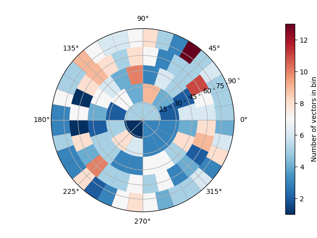
Looks like strong alignment in +Y and +X, although there really aren’t enough particles to be conclusive.

Label toolkit: Ellipse Axes

Given the moment of inertia results, a very convenient result from Ikeda et al., (2000) allows the a,b,c axes of the equivalent ellipsoid to be computed.

There is an option to strictly enforce the volume of the ellipse that we are not taking here.

ellipseDimensions = spam.label.ellipseAxes(labelled, volumes=volumes, MOIeigenValues=MOIeigenValues)
print(ellipseDimensions)

[[0.    0.    0.   ]
 [4.526 1.868 1.468]
 [4.257 3.585 2.691]
 ...
 [4.538 4.148 2.917]
 [4.236 2.282 1.976]
 [4.688 3.862 2.136]]

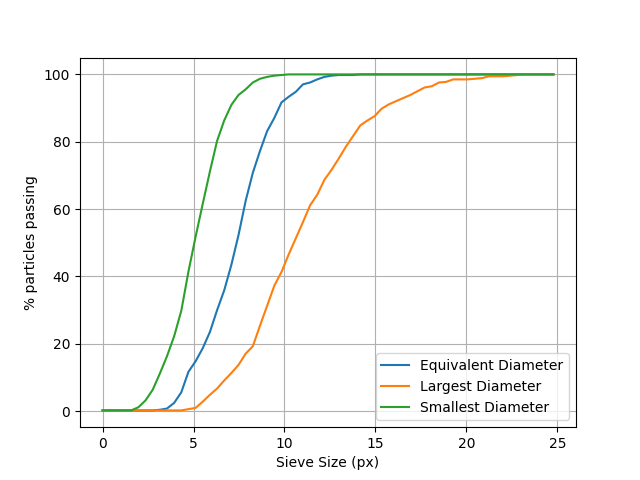
Label toolkit: Particle Size Distribution

We offer a tool to plot particle size distributions. Here we compute the equivalent-volume-sphere radii for each label and compare it to the distribution of largest and smallest ellipsoid axes as calculated above

equivalentRadii = spam.label.equivalentRadii(labelled, boundingBoxes=boundingBoxes)

# Run the particle size distribution plotter
spam.plotting.plotParticleSizeDistribution([equivalentRadii.tolist(),
                                            ellipseDimensions[:, 0].tolist(),
                                            ellipseDimensions[:, 2].tolist()], bins=64,
                                            legendNames=["Equivalent Diameter", "Largest Diameter", "Smallest Diameter"],
                                            cumulative=True)

plotParticleSizeDistribution(): Multiplying radii by two to make diameters
plotParticleSizeDistribution(): Multiplying radii by two to make diameters
plotParticleSizeDistribution(): Multiplying radii by two to make diameters

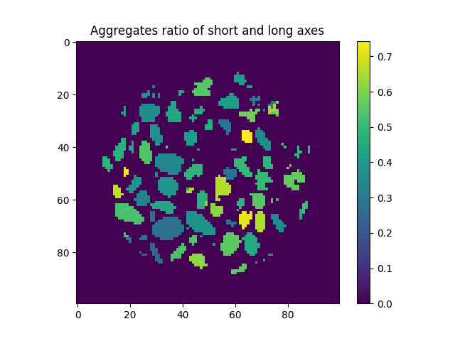
Label tookit: Showing scalars using labels

One convenient way in which to show results is to colour labels to represent some quantity. See Hall et al., (2010) for an early example. In this context we achieve this by converting a labelled image into an image where labels are replaced by some scalar.

Why don’t we colour grains by the ratio of their short and long axes?

ellipseDimensions = spam.label.ellipseAxes(labelled, volumes=volumes, MOIeigenValues=MOIeigenValues)
cOverA = ellipseDimensions[1:, 2] / ellipseDimensions[1:, 0]

plt.figure()
plt.title("Aggregates ratio of short and long axes")
plt.imshow(spam.label.convertLabelToFloat(labelled, cOverA)[midSlice])
plt.colorbar()

<matplotlib.colorbar.Colorbar object at 0x7f15b0b73d90>

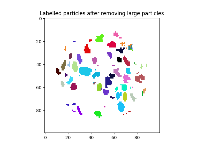
Label tookit: Removing labels

A common operation can be the removal of unwanted labels from a volume, either they are too small, or too large, or with some other undesired property.

Removing labels is not necessarily difficult, you can do: labelled[ labelled == unWantedLabel ] = 0

…however this is slow, and needs to be done for each unwanted label number. We offer a function that can quickly erase a list of labels. Since the outputs from the various spam.label functions are listed in contnunous label order, numpy.where will give us correct indices:

tooBigParticles = numpy.where(volumes > 500)
print(tooBigParticles)
labelled = spam.label.removeLabels(labelled, tooBigParticles)

(array([ 42,  57,  80,  92,  99, 101, 114, 116, 117, 119, 144, 183, 184,
       187, 200, 245, 246, 264, 267, 268, 285, 295, 305, 306, 308, 312,
       322, 365, 366, 370, 381, 391, 402, 445, 455, 461, 466, 474, 477,
       486, 487, 492, 518, 519, 535]),)

However now the labels are no longer continuous, so if we remove label 80 from the labelled volume, there is a gap! Labels go 78, 79, 81 82…

To avoid this we provide makeLabelsSequential

labelled = spam.label.makeLabelsSequential(labelled)
plt.figure()
plt.title("Labelled particles after removing large particles")
plt.imshow(labelled[midSlice], cmap=spam.label.randomCmap)

<matplotlib.image.AxesImage object at 0x7f15b0b70e50>

One common requirement is, when working with a subvolume, to remove labels on the edge of the cube, the labels are obtained with:

edgeLabels = spam.label.labelsOnEdges(labelled)
print(edgeLabels)
plt.show()

[0]

However here we don’t have any!