Kalisphera virtual concrete generation for multimodal registration

In this example we will read a series of sphere centres and radii coming from a DEM simulation and generate two voxelised images:

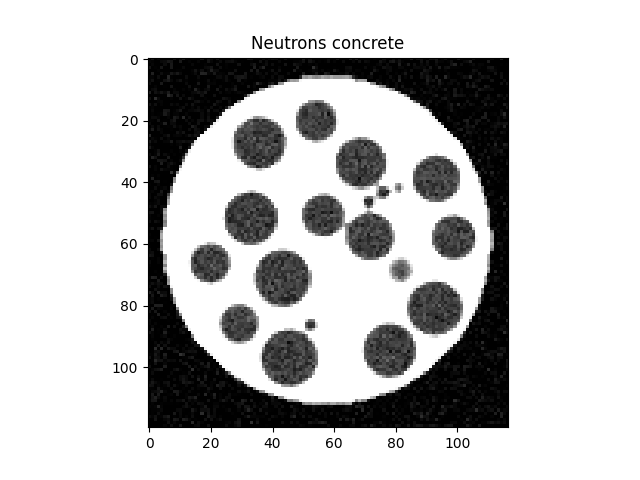
1. The first will correspond to a neutron concrete image

2. The second will correspond to an x-ray concrete image.

For both images, we will use Kalisphera to make a “perfect” rendering, which we will then degrade with blur and noise to make it look like a “real” tomography image. The technique is detailed in [Tengattini2015].

Note

The two images will not be aligned. The spheres of the neutron concrete image will be displaced to generate the x-ray concrete image. This is a very convenient starting point to then do a multimodal registration of the two images.

import numpy
import scipy.ndimage
import spam.datasets
import spam.deformation
import spam.mesh
import spam.kalisphera
import matplotlib.pyplot as plt
#import tifffile
#import spam.helpers

Create a helper function

First, we will need a helper function that creates the cylindrical virtual “concrete”:

def virtualConcrete(dims, phaseColours, positions1, radii1, positions2, radii2, cylinderRadius, cylinderCentre, cylinderHeight, gaussianBlur=0.8, gaussianNoise=0.2):
    """
    This function makes a z-aligned cylindrical virtual "concrete" with a matrix and embedded spheres
    of different colours. Background colour = 0.0.
    ``Kalisphera`` is used to make a "perfect" rendering of the spheres, which will then be degraded with blur and noise to make it look like a “real” tomography image

    Parameters:
    -----------
        dims : 3-component list of output dimensions

        phaseColours: 3-component list
            values for 3 phases: matrix, grains and pores

        positions1 : Nx3 numpy array
            positions of grain phase spheres

        radii1 : N numpy array
            radii of grain phase spheres

        positions2 : Nx3 numpy array
            positions of pores phase spheres

        radii2 : N numpy array
            radii of pores phase spheres

        cylinderRadius : float

        cylinderCentre : 3-component list

        cylinderHeight : float


    Returns:
    --------
        imCyl : 3D numpy array
    """

    phaseOne = numpy.zeros(dims, dtype="<f8")
    phaseTwo = numpy.zeros(dims, dtype="<f8")

    # TODO top and bottom crop
    imCyl = (spam.mesh.createCylindricalMask(dims, cylinderRadius, centre=cylinderCentre[1:]) * phaseColours[0]).astype('<f8')

    spam.kalisphera.makeSphere(phaseOne, positions1, radii1)
    spam.kalisphera.makeSphere(phaseTwo, positions2, radii2)

    # cleanup outside of balls
    phaseOne[imCyl==0] = 0
    phaseTwo[imCyl==0] = 0

    # Add in contributions
    imCyl += phaseOne * (phaseColours[1] - phaseColours[0])
    imCyl += phaseTwo * (phaseColours[2] - phaseColours[0])

    # brutally and horizontally slice the height limits
    imCyl[0:int(cylinderCentre[0]-cylinderHeight/2)]   = 0
    imCyl[  int(cylinderCentre[0]+cylinderHeight/2)::] = 0

    # Add gaussian (spatial) blur
    imCyl = scipy.ndimage.gaussian_filter(imCyl, sigma=gaussianBlur)
    # Add random noise
    imCyl = numpy.random.normal(imCyl, scale=gaussianNoise)

    return imCyl

Assign phase values

We assume that concrete is a three-phase material: mortar, grains, pores. To create the neutron and the x-ray concrete images, we will need to assign reasonable values for each phase imaged with the two modalities:

# Reasonable values for each phase of concrete
mortarX =  3     # X-ray  , mortar
mortarN =  5     # Neutron, mortar
grainsX =  5.2   # X-ray  , grains
grainsN =  0.2   # Neutron, grains
poresX  =  0.1   # X-ray  , pores
poresN  =  0.1   # Neutron, pores

We will then set the blur and noise levels to make these values look like a “real” tomography image

# The standard deviation of the image blurring to be applied first
blurSTD = 0.5
# The standard deviation of the random noise to be added to each voxel
noiseSTD = 0.05

Read input DEM data

We will now read the spheres positions and radii coming from a DEM simulation. These data will be the input for the neutron image:

spheres = spam.datasets.loadDEMspheresMMR()
pos = spheres[:, -2::-1] # swap z and x axis
radii = spheres[:, -1]

The DEM data is normally in SI units, so we need to define the pixel size for voxelisation:

pixelSizeM = 0.00005
posPx  = pos/pixelSizeM
radiiPx    = radii/pixelSizeM

We will set the dimensions of our cylinders and center the spheres to stick in the middle:

dims = (numpy.ceil(numpy.max(posPx, axis=0) - numpy.min(posPx, axis=0))*1.3).astype(int)
middle = (dims - 1) / 2.0
cylRadiusPx = min(dims[1:])*0.9/2.0

# Center the spheres and stick in middle of dims
posPx -= numpy.mean(posPx, axis=0)
posPx += middle

Create neutron image

We will now call the helper function to create the neutron image:

# Create the neutrons
neutrons = virtualConcrete(dims, [mortarN, grainsN, poresN],
                           posPx[radiiPx==radiiPx.max()], radiiPx[radiiPx==radiiPx.max()],
                           posPx[radiiPx==radiiPx.min()], radiiPx[radiiPx==radiiPx.min()],
                           cylRadiusPx, middle, dims[0]*0.9,
                           gaussianBlur=blurSTD, gaussianNoise=noiseSTD)
#tifffile.imwrite("Neutrons.tif", neutrons.astype('<f4'))

plt.figure()
plt.imshow(neutrons[neutrons.shape[0] // 2], vmin=0, vmax=1, cmap='Greys_r')
plt.title("Neutrons concrete")
plt.show()

Create x-ray image

We will now set the positions of the spheres for the x-ray image. For this, we will displace the spheres positions coming from the DEM simulation based on a deformation function that corresponds to a rigid body motion:

# move the grains according to the deformation function
Phi = spam.deformation.computePhi({'t': [0, 2, -1], 'r': [90, 0, 0]})

for i, poPx in enumerate(posPx):
    posPx[i] += spam.deformation.decomposePhi(Phi, PhiCentre=middle, PhiPoint=poPx)['t']

# moving the middle of the cylinder
middleMoved = middle + spam.deformation.decomposePhi(Phi)['t']

We will now call the helper function to create the x-rays image:

# Create the x-rays
xrays = virtualConcrete(dims, [mortarX, grainsX, poresX],
                        posPx[radiiPx==radiiPx.max()], radiiPx[radiiPx==radiiPx.max()],
                        posPx[radiiPx==radiiPx.min()], radiiPx[radiiPx==radiiPx.min()],
                        cylRadiusPx, middleMoved, dims[0]*0.9,
                        gaussianBlur=blurSTD, gaussianNoise=noiseSTD)
#tifffile.imwrite("Xrays.tif", xrays.astype('<f4'))

plt.figure()
plt.imshow(xrays[xrays.shape[0] // 2], vmin=0, vmax=5, cmap='Greys_r')
plt.title("X-rays concrete")
plt.show()

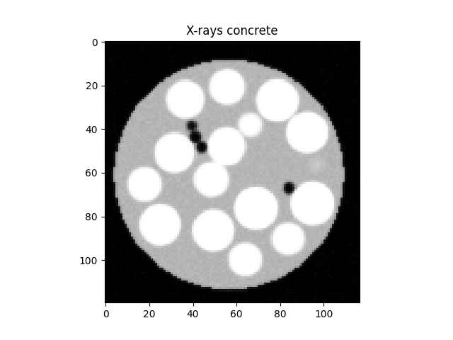
The datasets are ready!

Initial guess for multimodal registration

These two images can now be the input of a mulitmodal registration algorithm. To help this algorithm to converge, we can give a reasonable initial guess of the transformaion between these two images:

# PhiGuess: a bit off of the actual Phi that displaced the spheres
PhiGuess =  spam.deformation.computePhi({'t': [0, 1, 0], 'r': [91, 0, 0]})

We can now save this initial guess in a TSV file, to be a ready input for the mulitomodal registration algorithm:

# Creating a dictionary emulating a converged previous registration.
Reg = {}
Reg['Phi']          =  PhiGuess
Reg['error']        =  0.001
Reg['returnStatus'] =  2
Reg['iterations']   =  2
Reg['deltaPhiNorm'] =  0.01
#spam.helpers.writeRegistrationTSV('./guessPhiNtoX.tsv', middle, Reg)