Kalisphera sphere assembly generation

Here we want to read a series of sphere centres and radii (in this case from a DEM simulation) and generate a corresponding voxelised image.

We will use Kalisphera to make a “perfect” rendering, which we will then degrade with blur and noise to make it look like a “real” tomography image. The technique is detailed in [Tengattini2015]. This is a very convenient starting point to then do measurement tests on (contact detection, separation algorithms, discrete DIC, etc…)

import numpy
import math
import scipy.ndimage
import spam.datasets
import spam.kalisphera
import matplotlib.pyplot as plt

The DEM data is normally in SI units, so we need to define the pixel size for voxelisation

# m/pixel
pixelSize = 30.e-6
# The standard deviation of the image blurring to be applied first
blurSTD = 0.8
# The standard deviation of the random noise to be added to each voxel
noiseSTD = 0.03
boxSizeDEM, centres, radii = spam.datasets.loadDEMboxsizeCentreRadius()
# get maximum radius to pad our image (periodic boundaries...)
rMax = numpy.amax(radii)
boxSize = boxSizeDEM + 3 * rMax
# move the positions to the new center of the image
centres[:, :] = centres[:, :] + 1.5 * rMax
# turn the mm measures into pixels
boxSize = int(math.ceil(numpy.max(boxSize[:]) / pixelSize))
centres = centres / pixelSize
radii = radii / pixelSize

Allocate array of boxSize, The kalisphera C++ will fill this in…

Box = numpy.zeros((boxSize, boxSize, boxSize), dtype="<f8")
plt.figure()
plt.imshow(Box[Box.shape[0] // 2], vmin=0, vmax=1, cmap='Greys_r')
plt.title("Empty Array")
plt.show()

Call C++ function (Thanks Félix) This will sequentially add spheres into the array, the greylevel of the centre of the sphere will be 1.0

spam.kalisphera.makeSphere(Box, centres, radii)

0

Since the data comes from DEM, which uses small overlaps of particles to compute reaction forces, we might find pixels more than 100% full. We’ll just reset them to 1.

Box[numpy.where(Box > 1.0)] = 1.0
Box[numpy.where(Box < 0.0)] = 0.0
# Since we'd like [0, 1] greyvalues to be a normalised basis,
# we will move the pore value from 0 to 0.25 and the solid value
# from 1 to 0.75.
# This leaves a bit of data range in [0, 1] for the application of noise
Box = Box * 0.5
Box = Box + 0.25
plt.figure()
plt.imshow(Box[Box.shape[0] // 2], vmin=0, vmax=1, cmap='Greys_r')
plt.title("Kalisphera rescaled [0.25, 0.75]")
plt.show()

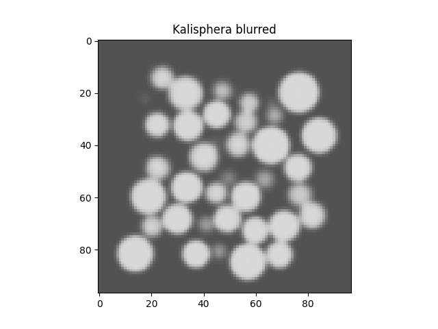
Add gaussian (spatial) blur. It is important for this to happen before adding random noise to each voxel since the gaussian blur is also a denoising operation (so you won’t get out the value of random noise you put in).

Box = scipy.ndimage.gaussian_filter(Box, sigma=blurSTD)
plt.figure()
plt.imshow(Box[Box.shape[0] // 2], vmin=0, vmax=1, cmap='Greys_r')
plt.title("Kalisphera blurred")
plt.show()

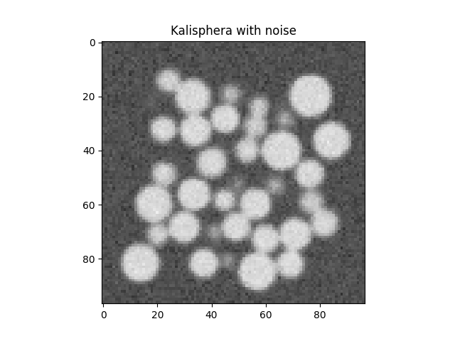
Now add random noise to each voxel. This perfectg dataset has now been “degraded” with the two most important/common sources of inaccuracies in tomographies

Box = numpy.random.normal(Box, scale=noiseSTD)
plt.figure()
plt.imshow(Box[Box.shape[0] // 2], vmin=0, vmax=1, cmap='Greys_r')
plt.title("Kalisphera with noise")
plt.show()